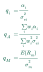
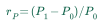

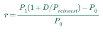

Combine price change and income over one holding period.
- P0,P1
- Beginning and ending prices
- I
- Cash income
- r
- Holding-period return
This browser version is too old for Quizara to display the page correctly. Update to the latest version and refresh to continue.
All formulas from the 2027 Level I course, organized by subject and Module, with explanations and worked examples for most formulas, free to use online.
Also used in this subject: EC · M8 · CF · M5 · EQ · M6 · EQ · M7 · FI · M6 · FI · M9 · DER · M10 · EQ · M12 · PM · M1 · PM · M2 · DER · M2 ·
| Formula | Equation | Details | ||||||||||||||||
|---|---|---|---|---|---|---|---|---|---|---|---|---|---|---|---|---|---|---|
Module 1 · Returns of Financial Assets and Instruments9 formulas | ||||||||||||||||||
Holding-period return (price, income, total; with reinvestment) | 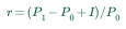 | |||||||||||||||||
Variants & steps (5)
What it meansCombine price change and income over one holding period.
Worked exampleMeasure the gain or loss from a price change alone.
Worked exampleMeasure distributions relative to the initial investment.
Worked exampleInclude shares acquired by reinvesting a dividend. Assumes one distribution, fractional reinvestment and no tax or costs.
Worked exampleMeasure total realized return over the investor's horizon.
Worked exampleSource Modules | ||||||||||||||||||
Arithmetic and geometric mean return |  | |||||||||||||||||
Variants & steps (2)
What it meansAverage observed periodic returns. The worked example below uses two periods.
Worked exampleFind the constant return with the same compounded growth. Each return must be at least -100%; growth factors must allow the stated root. The worked example below uses two periods.
Worked exampleSource Module | ||||||||||||||||||
Annualized return and CAGR | 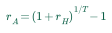 | |||||||||||||||||
Variants & steps (2)
What it meansConvert a holding-period return into an equivalent annual rate. Convert days to T using the stated day-count basis, such as days/360 or days/365. Do not mix conventions.
Worked exampleFind the constant yearly rate that connects a beginning value to an ending value. Positive starting and ending values; no intermediate cash flows. This is not the arithmetic mean of annual returns.
Worked exampleSource Modules | ||||||||||||||||||
Continuously compounded (log) return |  | |||||||||||||||||
Variants & steps (2)
What it meansExpress a price-only return using continuous compounding.
Worked exampleAdd log returns across successive periods.
Worked exampleSource Module | ||||||||||||||||||
Required / nominal expected return build-up | 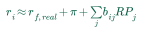 | |||||||||||||||||
Variants & steps (2)
What it meansBuild a required return from inflation and compensated risks. This is an additive approximation.
Worked exampleCombine real return, inflation and compensation for risk.
Worked exampleSource Module | ||||||||||||||||||
Excess return (arithmetic and compounded) |  | |||||||||||||||||
Variants & steps (2)
What it meansMeasure the return difference against a risk-free benchmark. The course defines compounded excess return as (1+ri)/(1+rf)−1. The arithmetic difference ri−rf is its approximation for small returns.
Worked exampleCompare wealth growth with a risk-free investment.
Worked exampleSource Module | ||||||||||||||||||
Real return (Fisher relation) |  | |||||||||||||||||
Variants & steps (3)
What it meansMeasure the change in purchasing power.
Worked exampleRemove inflation from the risk-free rate.
Worked exampleEstimate purchasing-power growth by subtracting inflation from the nominal return; the approximation is best for small rates. An approximation to the course’s exact Fisher relation; accurate when rates are small.
Worked exampleSource Module | ||||||||||||||||||
Gross, net and after-tax return |  | |||||||||||||||||
Variants & steps (3)
What it meansSeparate trading costs from investment gains.
Worked exampleCalculate the return remaining after investment fees.
Worked exampleApply different tax rates to realized gains and income. Assumes both components are taxed in the measured period.
Worked exampleSource Module | ||||||||||||||||||
Leveraged portfolio return | 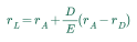 | |||||||||||||||||
Variants & steps (2)
What it meansMeasure the return on equity after financing an investment with debt. Single holding period, fixed beginning debt, no taxes or transaction costs; borrowing and asset returns cover the same period.
Worked exampleMeasure how borrowed funds amplify the spread between asset performance and financing cost. One period; fixed beginning debt, no taxes, fees, or interim cash flows. Losses can also be amplified. Notation: borrowed capital and equity correspond to the course’s leverage inputs; the borrowing rate is the interest paid on debt.
Worked exampleSource Module | ||||||||||||||||||
Module 2 · Types of Financial Returns1 formula | ||||||||||||||||||
Domestic-currency return on a foreign asset |  | |||||||||||||||||
Variants & steps (4)
What it meansCombine investment performance and the currency translation effect.
Worked exampleInclude both asset performance and exchange-rate movement.
Worked exampleMeasure the change in a price-per-base currency quote over a holding period. Keep the quote as domestic currency per unit of foreign currency for both dates.
Worked exampleCombine asset-return risk and exchange-rate risk, including their covariance, to estimate domestic-currency volatility.
Worked exampleSource Module | ||||||||||||||||||
Module 3 · Benchmarking Returns5 formulas | ||||||||||||||||||
Time-weighted return | 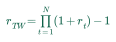 | |||||||||||||||||
Variants & steps (1)
What it meansLink returns while removing the effect of investor cash-flow timing.
Worked exampleSource Module | ||||||||||||||||||
Money-weighted return / IRR | 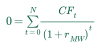 | |||||||||||||||||
Variants & steps (2)
What it meansFind the rate that balances dated contributions and withdrawals. Include ending investment value as a final positive investor cash flow.
Worked exampleFind the discount rate at which investment NPV is zero. Nonconventional cash flows can produce multiple or no IRRs.
Worked exampleSource Module | ||||||||||||||||||
Index weighting schemes |  | |||||||||||||||||
Variants & steps (5)
What it meansAssign weights in proportion to constituent market values.
Worked exampleExclude unavailable shares from capitalization weights.
Worked exampleWeight an index using a specified fundamental characteristic.
Worked exampleDetermine the relative exposure in a price-weighted index.
Worked exampleAllocate equally to all index constituents.
Worked exampleSource Module | ||||||||||||||||||
Index level and divisor (price-, value-, equal-weighted) |  | |||||||||||||||||
Variants & steps (3)
What it meansCalculate an index level from aggregate market capitalization.
Worked exampleCalculate a price-weighted index level. To preserve continuity at a stock split or other structural index change, divide the post-action price sum by the index level immediately before the action. This divisor adjustment offsets the corporate action at that instant; it must not remove ordinary market-price movements.
Worked exampleTrack an index that begins with equal investment in each constituent; rebalance to maintain equal weights. Choose share counts that create equal initial value weights; weights drift before rebalancing.
Worked exampleSource Module | ||||||||||||||||||
Price-return and total-return index | 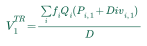 | |||||||||||||||||
Variants & steps (2)
What it meansInclude distributions when calculating the end value of a specified index basket. For an equal-weight starting basket, set fi=1 and use its constituent share quantities as Qi. Use a consistent basket and divisor; a continuing or rebalanced index must apply its own reinvestment, corporate-action and divisor rules.
Worked exampleMeasure each constituent’s price change and combine those returns using the index weights.
Worked exampleSource Module | ||||||||||||||||||
Module 4 · The Time Value of Money in Finance4 formulas | ||||||||||||||||||
PV and FV of a single cash flow (discrete, m-period, continuous) |  | |||||||||||||||||
Variants & steps (7)
What it meansMove a single amount forward through time. Each year's interest becomes part of the next year's starting amount. The worked example uses annual compounding at a constant rate and no additional deposits. Enter 6 for 6% in its input fields.
2027 scope note: 2027 scope: Quantitative Methods has a stronger applied focus, including interactive time-value-of-money lessons. This equation is not being labelled new. Worked exampleTranslate a future amount into today's money using a discount rate. The example uses annual compounding. In the general formula, r is the rate per period and N is the number of matching periods.
Worked exampleDiscount the only cash flow of a zero-coupon bond: its payment at maturity. Annual effective yield, no interim coupons, and the stated maturity payment is received.
Worked exampleApply a quoted annual rate with its stated compounding frequency.
Worked exampleGrow a cash amount at a continuous rate.
Worked exampleDiscount a payment using continuous compounding.
Worked exampleValue a combined stream by adding component values.
Source Module | ||||||||||||||||||
Effective annual rate and periodicity conversion | 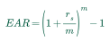 | |||||||||||||||||
Variants & steps (2)
What it meansInclude compounding within the year when comparing stated annual interest rates. The stated rate is nominal. Compounding periods must be a positive whole number.
Worked exampleCompare quoted yields on the same effective annual basis.
Worked exampleSource Modules | ||||||||||||||||||
Annuities: PV, FV, payment (ordinary and due) | 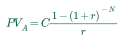 | |||||||||||||||||
Variants & steps (5)
What it meansDiscount a series of equal payments. At r=0 the limit is NC.
Worked exampleFind the payment that repays principal and interest. Payments arrive at period-end; at r=0 use PV/N.
Worked exampleValue a level payment stream whose first payment is today. Derived from ordinary-annuity present value by moving every payment one period earlier. At r=0, PV=N×PMT. Use BEGIN mode on a financial calculator.
Worked exampleAccumulate equal end-of-period payments at a constant rate to the final payment date.
Worked exampleAccumulate equal beginning-of-period payments; each payment earns one more period of interest than an ordinary annuity.
Worked exampleSource Module | ||||||||||||||||||
Level perpetuity |  | |||||||||||||||||
Variants & steps (1)
What it meansValue equal payments continuing indefinitely.
Worked exampleSource Module | ||||||||||||||||||
Module 5 · Statistical Characteristics of Asset Returns8 formulas | ||||||||||||||||||
Median and percentile location |  | |||||||||||||||||
Variants & steps (4)
What it meansLocate the middle observation after sorting.
Worked exampleAverage the two central ordered observations.
Worked exampleInterpolate between adjacent empirical observations, or between benchmark yields at neighboring maturities. For yield interpolation, p represents maturity and x represents the corresponding yield. Percentile conventions vary; use the stated method.
Worked exampleMeasure the spread of the middle half of observations as the third quartile minus the first.
Worked exampleSource Module | ||||||||||||||||||
Range and absolute deviation |  | |||||||||||||||||
Variants & steps (3)
What it meansMeasure the total spread of a sample.
Worked exampleAverage absolute distances from the mean.
Worked exampleMeasure dispersion with less sensitivity to extreme observations.
Worked exampleSource Module | ||||||||||||||||||
Variance and standard deviation (population and sample) | 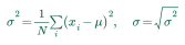 | |||||||||||||||||
Variants & steps (2)
What it meansMeasure dispersion when the observations are the entire population. Notation: N is the number of observations in the full population, denoted n in some course equations.
Worked exampleEstimate population dispersion from a sample. N must exceed 1.
Worked exampleSource Module | ||||||||||||||||||
Semivariance and target downside deviation | 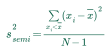 | |||||||||||||||||
Variants & steps (2)
What it meansMeasure squared deviations below the mean. The denominator uses the total sample size, not only below-mean observations.
Worked exampleMeasure downside deviations relative to a chosen return target.
Worked exampleSource Module | ||||||||||||||||||
Coefficient of variation |  | |||||||||||||||||
Variants & steps (1)
What it meansCompare dispersion relative to the mean. Most useful with a positive nonzero mean.
Worked exampleSource Modules | ||||||||||||||||||
Sample skewness and excess kurtosis | 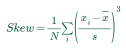 | |||||||||||||||||
Variants & steps (2)
What it meansDescribe asymmetry using standardized third moments. This is the unadjusted convention; software may apply a finite-sample correction.
Worked exampleCompare standardized fourth moments with the normal-distribution benchmark. The course uses this unadjusted convention for large samples (n ≥ 100). The small default example illustrates the arithmetic, not an unbiased small-sample estimate.
Worked exampleSource Module | ||||||||||||||||||
Covariance and correlation | 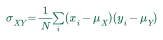 | |||||||||||||||||
Variants & steps (4)
What it meansMeasure whether two variables move together.
Worked exampleNormalize covariance to a value between -1 and 1.
Worked exampleTranslate a correlation estimate into covariance.
Worked exampleMeasure how two samples move together, then standardize covariance by their sample standard deviations.
Worked exampleSource Module | ||||||||||||||||||
Scaling variance and volatility across horizons | 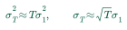 | |||||||||||||||||
Variants & steps (1)
What it meansScale risk across horizons under uncorrelated, identically distributed returns.
Worked exampleSource Module | ||||||||||||||||||
Module 6 · Statistical Distributions for Financial Asset Prices and Returns13 formulas | ||||||||||||||||||
CDF, density and interval probability |  | |||||||||||||||||
Variants & steps (4)
What it meansFind the probability of an outcome at or below a threshold.
Measure the probability over a continuous interval.
Worked exampleAdd probabilities of the outcomes inside an interval.
Worked exampleTranslate a smooth cumulative distribution into its density.
Source Module | ||||||||||||||||||
Expected value and scenario-weighted value |  | |||||||||||||||||
Variants & steps (5)
What it meansAverage possible outcomes using their probabilities. The probabilities must sum to 1.
Worked exampleCalculate a mean from a continuous distribution.
Combine any number of mutually exclusive valuation outcomes. Probabilities sum to 1 and values share a valuation date.
Worked exampleCombine downside, base, and upside valuation scenarios instead of relying on one outcome. Values are measured at the same date. The three scenario probabilities are non-negative and sum to 100%.
2027 scope note: 2027 scope: Probability-weighted scenarios are introduced as standard valuation practice in Equities. This is a coverage change, not a newly invented formula. Worked exampleCombine survival and distress valuation outcomes.
Worked exampleSource Module | ||||||||||||||||||
Variance and covariance of random variables | ![Var(X) = E(X^2) − [E(X) ]^2](/resources/formula-equations/20e1f51b1ebfc08f.svg) | |||||||||||||||||
Variants & steps (4)
What it meansMeasure uncertainty using first and second moments.
Worked exampleMeasure joint variation using expectations.
Worked exampleWeight squared deviations and paired deviations by scenario probabilities to measure risk and joint variation.
Worked exampleCombine asset returns within each scenario, then use scenario probabilities to calculate portfolio expected return and variance.
Worked exampleSource Module | ||||||||||||||||||
Binomial distribution and binomial tree | 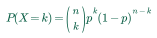 | |||||||||||||||||
Variants & steps (5)
What it meansCalculate exact and cumulative probabilities of binary outcomes.
Worked exampleDescribe the distribution of successes across repeated trials.
Worked exampleEvaluate binomial asymmetry and tail shape. Requires 0 < p < 1.
Worked exampleCalculate a price reached after a sequence of binomial moves.
Worked exampleApproximate binomial probabilities with a normal distribution when both expected successes and failures are sufficiently large; apply a continuity correction. Use a large trial count and probabilities away from the boundaries.
Worked exampleSource Module | ||||||||||||||||||
Poisson distribution | 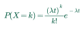 | |||||||||||||||||
Variants & steps (3)
What it meansModel the count of independent arrivals at a constant rate.
Worked exampleFind the probability of at most k events.
Worked exampleDescribe event counts under an independent constant-rate arrival model.
Worked exampleSource Module | ||||||||||||||||||
Constant hazard: survival, default and waiting time |  | |||||||||||||||||
Variants & steps (2)
What it meansTranslate a constant hazard rate into survival and default probabilities.
Worked exampleFind the mean waiting time under an exponential distribution.
Worked exampleSource Module | ||||||||||||||||||
Uniform distribution (discrete and continuous) | 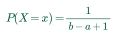 | |||||||||||||||||
Variants & steps (5)
What it meansModel equally likely integer outcomes. The CDF is zero below a and one at or above b.
Worked exampleDescribe dispersion and tail shape for a discrete uniform variable. Requires n greater than 1; unit spacing between outcomes.
Worked exampleFind the mean of a continuous uniform variable.
Worked exampleModel a continuously uniform outcome. Density is zero outside the interval; the CDF is clamped to zero or one there.
Worked exampleDescribe the spread and flat tails of a continuous uniform variable.
Worked exampleSource Module | ||||||||||||||||||
Normal distribution and standardization | ![f(x) = (1) / (σsqrt(2π)) exp [ − (1) / (2) ((x − μ) / (σ))^2]](/resources/formula-equations/372db4f03d9c8ed1.svg) | |||||||||||||||||
Variants & steps (3)
What it meansEvaluate a normal density at a specified outcome. Use a positive standard deviation. Course Module 6, Exhibit 19.
Worked exampleConvert an observation to a normal probability.
Worked exampleUse normal symmetry and tail shape as a benchmark.
Source Module | ||||||||||||||||||
Lognormal distribution |  | |||||||||||||||||
Variants & steps (5)
What it meansTranslate normal log parameters into a level mean.
Worked exampleMeasure variance in levels rather than logs.
Worked exampleCalculate probabilities for a positive lognormal variable. The outcome must be positive and log standard deviation must exceed zero. Course Module 6, Exhibit 19.
Worked exampleDescribe the right skew and heavy tails of lognormal levels.
Worked exampleModel a positive asset price by assuming its log return is normally distributed; scale drift and volatility to the horizon. This is the location of the log-price distribution, not a deterministic realized price.
Worked exampleSource Module | ||||||||||||||||||
Logistic distribution | 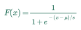 | |||||||||||||||||
Variants & steps (3)
What it meansModel a symmetric distribution with heavier tails than a normal distribution. The scale parameter must be positive. Course Module 6, Exhibit 19.
Worked exampleDescribe logistic symmetry and excess kurtosis.
Worked exampleFind the variance of a logistic variable.
Worked exampleSource Module | ||||||||||||||||||
Joint, marginal and total probability; independence | 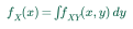 | |||||||||||||||||
Variants & steps (5)
What it meansIntegrate out the other variable.
Express independence through factorization of cumulative probabilities.
Find the joint probability that both continuous outcomes lie below thresholds.
Obtain the probability that both events occur.
Worked exampleCombine conditional event probabilities across all mutually exclusive scenarios. For the two-part case, use event B and its complement. The sum also applies to any finite partition; prior probabilities must add to one.
Worked exampleSource Module | ||||||||||||||||||
Conditional expectation and total expectation |  | |||||||||||||||||
Variants & steps (5)
What it meansAverage outcomes using conditional probabilities.
Worked exampleCalculate a continuous mean after observing another variable.
Measure remaining uncertainty after conditioning.
Worked exampleMeasure joint variation within a scenario.
Worked exampleCombine scenario-specific means into an unconditional mean.
Worked exampleSource Module | ||||||||||||||||||
Bayes' formula | 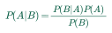 | |||||||||||||||||
Variants & steps (2)
What it meansUpdate an event probability after receiving evidence. P(B) must be positive.
Worked exampleUpdate a pattern's credibility after observing data. The same Bayes relationship applies to probabilities throughout the curriculum.
Worked exampleSource Module | ||||||||||||||||||
Module 7 · Estimation and Hypothesis Testing9 formulas | ||||||||||||||||||
Standard error and z confidence interval for the mean |  | |||||||||||||||||
Variants & steps (3)
What it meansMeasure variability of a sample mean.
Worked exampleStandardize a mean under normality or a suitable large-sample approximation.
Worked exampleConstruct a normal-theory mean interval when population volatility is known. Use population σ when known. For a sufficiently large sample, the course uses sample s with the z critical value under the central limit theorem (Module 7, Equations 3–4).
Worked exampleSource Module | ||||||||||||||||||
One-sample t-test for the mean and p-values |  | |||||||||||||||||
Variants & steps (5)
What it meansTest a population mean when its variance is estimated. Degrees of freedom N-1; normal-population assumptions matter for small samples.
Worked exampleMeasure the probability of a result at least as extreme in either tail.
Worked exampleEvaluate an upper-tail alternative with a continuous null distribution.
Worked exampleEvaluate a lower-tail alternative.
Worked exampleRelate test power to the probability of a Type II error and confidence level to the chosen significance level.
Worked exampleSource Module | ||||||||||||||||||
Two-sample (pooled-variance) t-test | 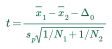 | |||||||||||||||||
Variants & steps (2)
What it meansCompare two means assuming equal population variances. Degrees of freedom N1+N2-2.
Worked examplePool variance estimates for an equal-variance two-sample t test.
Worked exampleSource Module | ||||||||||||||||||
Paired-difference t-test |  | |||||||||||||||||
Variants & steps (1)
What it meansTest a mean difference for paired observations.
Worked exampleSource Module | ||||||||||||||||||
Chi-square test of a single variance |  | |||||||||||||||||
Variants & steps (1)
What it meansTest a normal population's variance. Degrees of freedom N-1.
Worked exampleSource Module | ||||||||||||||||||
F-test of two variances |  | |||||||||||||||||
Variants & steps (1)
What it meansCompare variances of two normal populations. Put the larger sample variance in the numerator and use an upper-tail F critical value, with the matching numerator and denominator degrees of freedom.
Worked exampleSource Module | ||||||||||||||||||
Correlation tests (Pearson and Spearman) |  | |||||||||||||||||
Variants & steps (3)
What it meansTest zero population correlation under the appropriate distribution assumptions. Degrees of freedom N-2. Notation: r is the sample correlation denoted rXY in the course; N is the number of paired observations.
Worked exampleCalculate a correlation-test statistic from a Spearman rank coefficient. Use a Student t approximation with N−2 degrees of freedom for N>30. Small samples need specialized critical values. At an exactly perfect rank correlation, the finite statistic is undefined.
Worked exampleMeasure monotonic association using paired observation ranks. The displayed shortcut assumes no tied ranks. With ties, assign average ranks and take their Pearson correlation; the calculator implements this rank-correlation definition.
Worked exampleSource Module | ||||||||||||||||||
Chi-square test of independence | 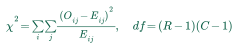 | |||||||||||||||||
Variants & steps (3)
What it meansTest whether row and column categories are independent. Degrees of freedom (rows-1)(columns-1); expected counts must support the approximation.
Worked exampleFind expected counts under independence.
Worked exampleIdentify cells contributing strongly to a chi-square statistic.
Worked exampleSource Module | ||||||||||||||||||
Parametric VaR |  | |||||||||||||||||
Variants & steps (1)
What it meansEstimate a normal-return loss quantile. Course Quant Module 7, Equation 5, assumes zero mean return for the holding period. PM Module 6 explains the loss amount, horizon and confidence level.
Worked exampleSource Modules | ||||||||||||||||||
Module 8 · The Return and Risk of a Financial Portfolio4 formulas | ||||||||||||||||||
Portfolio return (weighted; buy-and-hold vs rebalanced) | ![r_(P, T) = ∑_(i) w_(i, 0) [∏_(t = 1)^(T) (1 + r_(i, t)) − 1]](/resources/formula-equations/0bfb610b4bd151e1.svg) | |||||||||||||||||
Variants & steps (4)
What it meansCalculate a portfolio return without interim rebalancing.
Worked exampleCompound returns when weights can change between periods.
Worked exampleCombine asset expected returns on one horizon. The worked example below uses two assets.
Worked exampleAggregate asset returns with matching beginning weights.
Worked exampleSource Module | ||||||||||||||||||
Portfolio variance and standard deviation | 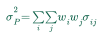 | |||||||||||||||||
Variants & steps (5)
What it meansInclude all variances and covariances in portfolio risk.
Worked exampleCalculate risk compactly for many assets. Optional matrix notation in the course.
Worked exampleMeasure total portfolio variance, including every cross term.
Worked exampleMeasure two-asset portfolio risk. Weights sum to one; borrowing or shorts can make weights fall outside zero to one. The worked example below uses two assets.
Worked exampleCount the distinct off-diagonal covariance inputs needed for portfolio risk. A symmetric covariance matrix has N individual variances and N(N−1)/2 distinct cross-asset covariances. The same covariance appears on both sides of the diagonal, so count each asset pair once.
Worked exampleSource Module | ||||||||||||||||||
Two-asset minimum-variance and target-return weights | 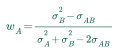 | |||||||||||||||||
Variants & steps (3)
What it meansFind the unconstrained minimum-variance allocation. Weight in B is 1-wA. Long-only constraints can move the optimum to a boundary.
Worked exampleSolve a two-asset allocation for a specified return. The two expected returns must differ.
Worked exampleCalculate two-asset portfolio variance for a chosen expected return using the course’s return-based weights; asset expected returns must differ.
Worked exampleSource Module | ||||||||||||||||||
Mean-variance utility | 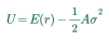 | |||||||||||||||||
Variants & steps (2)
What it meansCompare portfolios using a mean-variance preference model.
Worked exampleCompare strategic allocations under a stated risk penalty. The risk penalty coefficient λ here corresponds to A/2 in the Module 1 convention U = E(R) − (A/2)σ².
Worked exampleSource Modules | ||||||||||||||||||
Module 9 · Simulation of Financial Asset Prices and Returns1 formula | ||||||||||||||||||
Monte Carlo price simulation steps |  | |||||||||||||||||
Variants & steps (5)
What it meansGenerate a risk-neutral log-return step under geometric Brownian motion.
Worked exampleAdvance a risk-neutral geometric-Brownian-motion price path. This form assumes a non-dividend-paying asset. Use a consistent annual rate, volatility and time fraction.
Worked exampleGenerate two normal shocks with specified correlation.
Worked exampleConvert a simulated log return into a currency gain or loss.
Worked exampleCalculate the course’s Asian call payoff as the positive difference between the terminal price and the average path price. The course simulation example uses a floating-strike Asian call with the path-average price as strike.
Worked exampleSource Module | ||||||||||||||||||
Module 10 · Applications of Simple Linear Regression in Finance6 formulas | ||||||||||||||||||
Simple linear regression: model and OLS estimates | 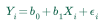 | |||||||||||||||||
Variants & steps (6)
What it meansExpress a linear relationship with an unexplained component.
Worked examplePredict the dependent variable from a fitted line.
Worked exampleMeasure the observation's unexplained component.
Worked exampleEstimate the least-squares slope. The predictor must have positive variation.
Worked examplePosition the fitted line through the sample means.
Worked exampleEstimate least-squares coefficients using matrix algebra. Optional matrix notation in the course; the scalar OLS formulas give the same estimates.
Worked exampleSource Module | ||||||||||||||||||
Sums of squares and R-squared |  | |||||||||||||||||
Variants & steps (6)
What it meansCalculate the share of variation explained by a regression with an intercept.
Worked exampleMeasure total dependent-variable variation.
Worked exampleMeasure variation explained by the fitted line.
Worked exampleMeasure squared residual variation.
Worked exampleSeparate explained and unexplained variation. Applies to OLS with an intercept.
For simple regression with an intercept, square the sample correlation to obtain the fraction of dependent-variable variation explained. Simple ordinary least squares regression with an intercept.
Worked exampleSource Module | ||||||||||||||||||
Standard error of estimate and F-test | 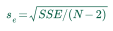 | |||||||||||||||||
Variants & steps (3)
What it meansEstimate residual volatility in simple regression with an intercept.
Worked exampleTest the joint significance of regression slopes.
Worked exampleEstimate disturbance variance. For simple regression k=1.
Worked exampleSource Module | ||||||||||||||||||
Tests and intervals for regression coefficients |  | |||||||||||||||||
Variants & steps (5)
What it meansTest a regression slope. Simple-regression degrees of freedom are N-2.
Worked exampleMeasure uncertainty in the fitted slope.
Worked exampleForm a two-sided confidence interval for a regression slope using its standard error. Use the critical value for the stated confidence level and regression degrees of freedom. Simple OLS with an intercept has df=N−2. The t interval relies on the corresponding regression-inference assumptions.
Worked exampleMeasure uncertainty in the fitted intercept.
Worked exampleCompare an estimated intercept with its hypothesized value in units of its standard error. Simple regression uses n−2 degrees of freedom.
Worked exampleSource Module | ||||||||||||||||||
Prediction interval for a new observation | 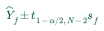 | |||||||||||||||||
Variants & steps (2)
What it meansForm a two-sided interval for one new response under a simple linear regression model. Use the new-observation prediction standard error, including residual uncertainty; this is wider than an interval for the mean response.
Worked exampleAccount for both fitted-line uncertainty and a new observation's disturbance.
Worked exampleSource Module | ||||||||||||||||||
Log-linear, linear-log and log-log regressions | 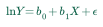 | |||||||||||||||||
Variants & steps (3)
What it meansModel proportional changes in Y from unit changes in X.
Worked exampleModel level changes in Y from proportional changes in X.
Worked exampleEstimate elasticity using a regression slope.
Worked exampleSource Module | ||||||||||||||||||
Also used in this subject: EQ · M8 ·
| Formula | Equation | Details | ||||||||||||||
|---|---|---|---|---|---|---|---|---|---|---|---|---|---|---|---|---|
Module 1 · The Firm and Market Structures5 formulas | ||||||||||||||||
Total and average costs |  | |||||||||||||||
Variants & steps (2)
What it meansCombine fixed and output-dependent production costs.
Worked exampleExpress production costs per unit. Q must be positive.
Worked exampleSource Module | ||||||||||||||||
Marginal revenue, marginal cost and MR = MC |  | |||||||||||||||
Variants & steps (2)
What it meansCompare the revenue and cost from additional output.
Worked exampleLocate an interior optimum when the cost and revenue curves support a maximum.
Source Module | ||||||||||||||||
Economic profit |  | |||||||||||||||
Variants & steps (1)
What it meansMeasure revenue remaining after all economic costs.
Worked exampleSource Module | ||||||||||||||||
Breakeven and shutdown conditions |  | |||||||||||||||
Variants & steps (2)
What it meansCompare operating revenue with avoidable variable costs in a short-run shutdown decision. Assumes fixed costs are unavoidable in the short run. Revenue above variable cost contributes toward fixed costs; equality is the shutdown boundary, and a firm may continue operating at this short-run boundary. Long-run viability requires covering total economic cost. For a perfectly competitive firm, the shutdown price is minimum AVC.
Identify output at which a firm earns zero economic profit. For positive output, divide total revenue and total cost by the same quantity. Zero economic profit includes a normal return on capital; accounting profit may still be positive. This is a condition to evaluate at a chosen output, not a formula that determines output without revenue and cost functions.
Source Module | ||||||||||||||||
Market share, concentration ratio and HHI |  | |||||||||||||||
Variants & steps (4)
What it meansMeasure the combined share of leading firms.
Worked exampleSum squared market shares of the top N firms, or all firms. An N-firm HHI uses only the selected N firms. The all-firm HHI uses every firm. Shares entered as percentages are converted to fractions; this result uses the 0–1 scale.
Worked exampleMeasure industry concentration on the zero-to-10,000 convention.
Worked exampleMeasure a company's share of its addressable industry.
Worked exampleSource Module | ||||||||||||||||
Module 2 · Understanding Business Cycles1 formula | ||||||||||||||||
Output gap (deviation from trend) | 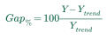 | |||||||||||||||
Variants & steps (1)
What it meansMeasure the output gap used to describe the growth cycle. Output is expressed as a percentage deviation from its trend. Positive means output is above trend, and negative means below trend. The choice of trend estimate affects the result; use matching units and price bases.
Worked exampleSource Module | ||||||||||||||||
Module 3 · Fiscal Policy1 formula | ||||||||||||||||
Budget balance, disposable income and fiscal multiplier |  | |||||||||||||||
Variants & steps (4)
What it meansCalculate disposable income in a simple proportional-tax model.
Worked exampleEstimate output response to government spending in the stated simple closed-economy model. Assumes no additional import leakage or interest-rate crowding out.
Worked exampleCalculate net government borrowing in a simple budget identity. Positive means a deficit; negative means a surplus. B denotes transfer spending.
Worked exampleEstimate the output effect of equal increases in government spending and taxes; in the simple model the multiplier is one. The course’s simple balanced-budget result assumes equal increases in spending and tax revenue.
Worked exampleSource Module | ||||||||||||||||
Module 4 · Monetary Policy1 formula | ||||||||||||||||
Neutral policy rate |  | |||||||||||||||
Variants & steps (1)
What it meansAdd real trend growth and long-run expected inflation to estimate the neutral rate. A higher policy rate is contractionary; a lower rate is expansionary. The neutral rate combines the course’s real trend growth and long-run expected inflation components.
Worked exampleSource Module | ||||||||||||||||
Module 6 · International Trade1 formula | ||||||||||||||||
Tariff revenue and deadweight loss |  | |||||||||||||||
Variants & steps (2)
What it meansCalculate the tariff revenue rectangle.
Worked exampleEstimate production and consumption distortions from a tariff. Linear supply and demand and a small-country setup.
Worked exampleSource Module | ||||||||||||||||
Module 7 · Capital Flows and the FX Market3 formulas | ||||||||||||||||
Real exchange rate |  | |||||||||||||||
Variants & steps (3)
What it meansAdjust a nominal currency quote for relative price levels.
Worked exampleSeparate currency movement from inflation effects.
Worked exampleAdjust the nominal quote change for inflation in the base and price currencies to measure the real exchange-rate change.
Worked exampleSource Module | ||||||||||||||||
Trade balance identity X - M = (S - I) + (T - G) |  | |||||||||||||||
Variants & steps (1)
What it meansConnect the trade balance with private and government saving.
Source Module | ||||||||||||||||
Percentage change in a currency | 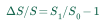 | |||||||||||||||
Variants & steps (2)
What it meansMeasure appreciation of the base currency in the stated quote.
Worked exampleMeasure appreciation or depreciation of the price currency by taking the reciprocal of the price-per-base quote. Reversing a quote requires taking its reciprocal; the two percentage changes are not exact negatives.
Worked exampleSource Module | ||||||||||||||||
Module 8 · Exchange Rate Calculations2 formulas | ||||||||||||||||
Cross rates and inverse quotes |  | |||||||||||||||
Variants & steps (2)
What it meansCombine two compatible currency quotes.
Worked exampleReverse the base and price currency of a quote.
Worked exampleSource Module | ||||||||||||||||
Forward exchange rate (covered interest parity, points, premium) | 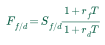 | |||||||||||||||
Variants & steps (6)
What it meansCalculate a no-arbitrage FX forward quote. Quote f/d means price currency f per unit of base currency d. Put the price-currency rate in the numerator and base-currency rate in the denominator; rates and year fraction must use matching conventions.
Worked exampleFind the forward-minus-spot adjustment under covered parity. Quote f/d means price currency f per unit of base currency d. Put the price-currency rate in the numerator and base-currency rate in the denominator; rates and year fraction must use matching conventions.
Worked examplePrice a currency forward using its explicit quote direction.
Worked exampleConvert forward points to a full outright forward quote. Often k = 10000; use the convention for the currency pair, including two-decimal JPY quotes.
Worked exampleInterpret the forward premium as an expected spot change under the forward-as-expected-spot assumption. Assumes Ft=Et[St+1] for the foreign-per-domestic quote. This expected-spot interpretation is an additional modeling assumption; historical forward rates have large forecast errors. Rates use the same horizon.
Worked exampleCompare the forward quote with spot; covered interest parity relates the premium or discount to the two currency interest rates. This is a covered-interest-parity premium; it does not require a forward-as-expected-spot assumption.
Worked exampleSource Modules | ||||||||||||||||
| Formula | Equation | Details | ||||||||||
|---|---|---|---|---|---|---|---|---|---|---|---|---|
Module 1 · Organizational Forms, Corporate Issuer Features, and Ownership1 formula | ||||||||||||
Combined corporate and dividend tax rate | 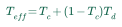 | |||||||||||
Variants & steps (1)
What it meansMeasure total tax on fully distributed corporate earnings.
Worked exampleSource Module | ||||||||||||
Module 4 · Working Capital and Liquidity3 formulas | ||||||||||||
Working capital and cash conversion cycle |  | |||||||||||
Variants & steps (2)
What it meansMeasure the time between operating cash payments and receipts.
Worked exampleDistinguish current assets minus current liabilities from the narrower operating working-capital measure used in cash-flow analysis.
Worked exampleSource Module | ||||||||||||
Cost of forgoing a supplier discount | 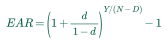 | |||||||||||
Variants & steps (1)
What it meansAnnualize the cost of paying at the later deadline. N must exceed D; use the specified day-count year.
Worked exampleSource Module | ||||||||||||
Free cash flow after capital investment |  | |||||||||||
Variants & steps (1)
What it meansMeasure operating cash left after investment in long-term assets. This liquidity measure is distinct from valuation FCFF and FCFE; it makes no additional financing or after-tax interest adjustment.
Worked exampleSource Module | ||||||||||||
Module 5 · Capital Investments and Capital Allocation3 formulas | ||||||||||||
ROIC and its margin-turnover decomposition | 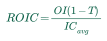 | |||||||||||
Variants & steps (2)
What it meansCompare after-tax operating profit with its supporting capital.
Worked exampleSeparate operating profitability and capital efficiency.
Worked exampleSource Module | ||||||||||||
Net present value | 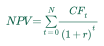 | |||||||||||
Variants & steps (2)
What it meansValue an investment's full cash-flow stream in today's money. Cash outflows are negative; use a discount rate appropriate to the cash flows.
Worked exampleSubtract the investment outlay from the present value of its expected cash inflows. The initial outlay is entered as a positive amount; C1 and C2 arrive at each year-end. Use a discount rate appropriate to the cash flows.
Worked exampleSource Modules | ||||||||||||
After-tax cash flow with depreciation tax shield |  | |||||||||||
Variants & steps (1)
What it meansAdjust a taxable operating cash flow for tax and any deductible depreciation shield. Noncash depreciation affects operating cash flow through tax deductions. Without a depreciation deduction, the adjustment reduces to CF×(1−T). Assumes deductions can be used in the period. Do not apply this rule to an initial investment, untaxed receipts, working-capital movements or disposal proceeds without their separate tax treatment.
Worked exampleSource Module | ||||||||||||
Module 6 · Capital Structure4 formulas | ||||||||||||
MM Proposition I and trade-off firm value |  | |||||||||||
Variants & steps (4)
What it meansExpress capital-structure irrelevance under the no-tax MM assumptions.
Add the value of a perpetual debt tax shield. Uses the standard MM assumptions and a permanent debt policy. Notation: T denotes the corporate tax rate written as t in the course.
Worked exampleBalance tax benefits against expected financial-distress costs.
Worked exampleCalculate debt interest under a constant-rate model.
Worked exampleSource Module | ||||||||||||
MM Proposition II (cost of equity) | 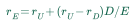 | |||||||||||
Variants & steps (2)
What it meansMeasure financial leverage's effect under the no-tax MM model.
Worked exampleEstimate the required equity return with a debt tax shield. Notation: T is the course tax rate t; the unlevered cost of equity corresponds to the course’s required return on an unlevered firm.
Worked exampleSource Module | ||||||||||||
WACC and capital weights |  | |||||||||||
Variants & steps (3)
What it meansCombine the required returns on debt and equity, allowing for the debt interest tax shield. Debt and equity only; market-value weights total 100%. Interest is fully tax-deductible at the stated tax rate.
Worked exampleCalculate funding weights for a two-source capital structure.
Worked exampleCombine all capital providers' required returns. Weights sum to one; the interest tax shield must apply. Debt, preferred-equity and common-equity weights add to one; their component costs correspond to the course’s financing costs.
Worked exampleSource Module | ||||||||||||
Operating and financial leverage |  | |||||||||||
Variants & steps (3)
What it meansMeasure the sensitivity of net income to a change in operating income. Use comparable relative changes over the same period; a zero operating-income change makes the ratio undefined. This sensitivity measure differs from the assets-to-equity multiplier.
Worked exampleMeasure fixed costs as a proportion of total operating costs. This ratio describes the operating cost structure. It differs from the degree of operating leverage, which measures the sensitivity of operating profit to sales. Use nonnegative costs on the same basis and activity range; total operating costs must be positive.
Worked exampleMeasure profit and its sensitivity to unit sales.
Worked exampleSource Module | ||||||||||||
| Formula | Equation | Details | ||||||||||||||||||||||||
|---|---|---|---|---|---|---|---|---|---|---|---|---|---|---|---|---|---|---|---|---|---|---|---|---|---|---|
Module 2 · Analyzing Income Statements3 formulas | ||||||||||||||||||||||||||
Basic EPS | 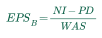 | |||||||||||||||||||||||||
Variants & steps (1)
What it meansCalculate earnings attributable to each common share.
Worked exampleSource Module | ||||||||||||||||||||||||||
Diluted EPS (if-converted and treasury stock method) | 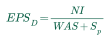 | |||||||||||||||||||||||||
Variants & steps (3)
What it meansCalculate if-converted EPS when preferred dividends are eliminated. This simplified formula assumes all preferred dividends are attributable to convertible preferred shares. With any non-convertible preferred shares, subtract their dividends from net income.
Worked exampleAdd back after-tax interest and assumed conversion shares. Exclude antidilutive instruments.
Worked exampleFind shares added by dilutive in-the-money options. Apply only when the exercise price is below the average market price.
Worked exampleSource Module | ||||||||||||||||||||||||||
Profit margins |  | |||||||||||||||||||||||||
Variants & steps (4)
What it meansMeasure profitability after product costs.
Worked exampleMeasure operating profit earned per unit of revenue.
Worked exampleMeasure the share of revenue retained as net income.
Worked exampleMeasure the share of revenue remaining after operating and financing costs, before income taxes.
Worked exampleSource Module | ||||||||||||||||||||||||||
Module 3 · Analyzing Balance Sheets2 formulas | ||||||||||||||||||||||||||
Book value of equity |  | |||||||||||||||||||||||||
Variants & steps (4)
What it meansDetermine equity as the residual accounting claim.
Worked exampleReconcile the resources of a business with creditor and owner claims. Book equity is the residual interest in assets after liabilities; use this as explanatory context for the book-equity calculation. Reconcile book equity from contributed capital, retained earnings and treasury stock. This simplified composition assumes other equity reserves are zero. Include accumulated other comprehensive income and other recognized equity accounts when they are present.
Worked exampleShow the book-equity amount after excluding recognized intangible assets. This is an analytical book-value adjustment, not a claim that intangibles have no economic value. Include goodwill once within the intangible total. Further tax and other adjustments may be required for a different definition of tangible equity.
Worked exampleSource Module | ||||||||||||||||||||||||||
Solvency (leverage) ratios |  | |||||||||||||||||||||||||
Variants & steps (4)
What it meansMeasure financial leverage using debt and equity balances.
Worked exampleAssess long-term debt relative to owners' capital.
Worked exampleMeasure the share of assets financed by debt.
Worked exampleMeasure the debt share of total debt and equity capital.
Worked exampleSource Module | ||||||||||||||||||||||||||
Module 4 · Analyzing Statements of Cash Flows I1 formula | ||||||||||||||||||||||||||
Operating cash flow (direct and indirect) and cash reconciliation |  | |||||||||||||||||||||||||
Variants & steps (8)
What it meansReconcile earnings to operating cash flow. Avoid counting the same noncash or nonoperating adjustment twice.
Worked exampleConvert revenue into customer cash receipts. Enter balance increases as positive and decreases as negative. Set the deferred-revenue change to zero when there are no customer advances. Assumes these balance changes arise only from the stated sales, advances and collections; write-offs, acquisitions and currency effects need separate adjustments.
Worked exampleConvert product costs into supplier cash payments.
Worked exampleReconcile accrued interest expense to cash paid for interest. Interest paid is reconciled with the change in interest payable. A decrease in interest payable increases cash paid. Assumes this account changes only through the stated expense and payments; other noncash or capitalized-interest adjustments require separate treatment.
Worked exampleAdjust other operating expenses for prepayments and unpaid accruals. Enter increases as positive and decreases as negative. Include only the prepaid and accrued accounts related to these expenses, and remove any noncash expense before this reconciliation. Assumes no other account movements.
Worked exampleConvert accrued salary and wage expense to employee cash payments. An increase in wages payable reduces cash paid relative to expense; a decrease raises it. Assumes the payable balance changes only through these expenses and payments.
Worked exampleBuild operating cash flow from cash receipts and cash payments. This presentation classifies investment interest, dividends received and interest paid as operating cash flows. Adjust the components if the reporting framework or issuer uses another permitted classification.
Worked exampleReconcile opening and closing cash using the three cash-flow categories. Use inflows as positive and outflows as negative on a common cash-definition basis. This simplified relationship excludes currency-translation and other reconciliation movements; include those separately when present. A negative forecast balance indicates a funding shortfall under the assumptions.
Worked exampleSource Module | ||||||||||||||||||||||||||
Module 5 · Analyzing Statements of Cash Flows II4 formulas | ||||||||||||||||||||||||||
Free cash flow to the firm |  | |||||||||||||||||||||||||
Variants & steps (7)
What it meansCalculate cash available to debt and equity capital providers.
Worked exampleConvert operating cash flow into cash for all funding providers. This form assumes interest paid is classified within CFO.
Worked exampleEstimate firm free cash flow from EBITDA.
Worked exampleEstimate operating earnings after tax before funding costs.
Worked exampleBuild after-tax operating profit from a detailed financial forecast.
Worked exampleCalculate the reinvestment deducted from after-tax operating earnings.
Worked exampleCombine working-capital and net long-term capital requirements.
Worked exampleSource Module | ||||||||||||||||||||||||||
Free cash flow to equity |  | |||||||||||||||||||||||||
Variants & steps (5)
What it meansMeasure cash available to common equity after investment and net borrowing. Assumes interest paid is already included in CFO. Under IFRS, if interest paid is classified in financing cash flow, subtract after-tax interest before applying this formula.
Worked exampleMeasure equity cash flow after investment and financing.
Worked exampleConvert firm cash flow into equity cash flow.
Worked exampleReconcile cash available to equity with uses of that cash.
Worked exampleEstimate cash flow available to equity when new debt finances a fixed share of net investment. Maintain the target financing ratio; net investment includes the working-capital change.
Worked exampleSource Modules | ||||||||||||||||||||||||||
Cash flow performance ratios |  | |||||||||||||||||||||||||
Variants & steps (4)
What it meansCompare operating cash generation with sales.
Worked exampleCompare operating cash generation with operating profit.
Worked exampleTrack the cash-flow support for reported earnings over time. Repeated ratios below one or a declining trend can be warning signals when net income is positive; investigate accruals and business conditions before drawing a conclusion. A zero denominator is undefined, and loss-making periods need separate interpretation. This ratio uses net income rather than operating income.
Worked exampleExpress cash generation attributable to common shares.
Worked exampleSource Module | ||||||||||||||||||||||||||
Cash flow coverage ratios |  | |||||||||||||||||||||||||
Variants & steps (6)
What it meansCompare annual operating cash with debt outstanding.
Worked exampleCompare operating cash with debt repayments.
Worked exampleCompare pre-interest, pre-tax operating cash with interest payments. Use compatible cash-flow classifications.
Worked exampleMeasure the capacity to fund capital investment from operations.
Worked exampleCompare cash generation with dividend payments.
Worked exampleCompare operating cash with investment and funding cash demands.
Worked exampleSource Module | ||||||||||||||||||||||||||
Module 6 · Analysis of Inventories2 formulas | ||||||||||||||||||||||||||
Inventory cost flow (COGS identity, weighted-average cost) |  | |||||||||||||||||||||||||
Variants & steps (2)
What it meansReconcile inventory purchases and cost recognition. FIFO assigns the oldest available costs to COGS and the newest costs to ending inventory. LIFO assigns the newest costs to COGS and the oldest costs to ending inventory; apply the course’s layer-allocation procedure.
Worked exampleAllocate inventory cost under the weighted-average method.
Worked exampleSource Modules | ||||||||||||||||||||||||||
Inventory at lower of cost or NRV |  | |||||||||||||||||||||||||
Variants & steps (1)
What it meansApply a lower-of-cost-or-net-realizable-value measurement. Applies under IFRS and applicable US GAAP inventory methods; LIFO and retail-method US GAAP rules differ.
Worked exampleSource Module | ||||||||||||||||||||||||||
Module 7 · Analysis of Long-Term Assets3 formulas | ||||||||||||||||||||||||||
Depreciation methods |  | |||||||||||||||||||||||||
Variants & steps (4)
What it meansAllocate depreciable cost evenly over useful life.
Worked exampleApply a constant accelerated rate to declining book value. For double-declining balance, q = 2/N. Apply the rate to opening book value without first deducting salvage value; stop depreciation at salvage value.
Worked exampleAllocate depreciable cost to each unit produced, then multiply by current-period production.
Worked exampleDouble the straight-line depreciation rate for declining-balance depreciation; do not depreciate below salvage value.
Worked exampleSource Module | ||||||||||||||||||||||||||
Estimated asset age and useful life |  | |||||||||||||||||||||||||
Variants & steps (3)
What it meansEstimate average asset age under straight-line depreciation. Assumes no salvage value and a comparable stable asset pool.
Worked exampleEstimate remaining useful life under the simple straight-line model.
Worked exampleEstimate the total life of an asset pool. Assumes straight-line depreciation and no salvage value.
Worked exampleSource Module | ||||||||||||||||||||||||||
Asset impairment (IFRS and US GAAP) |  | |||||||||||||||||||||||||
Variants & steps (2)
What it meansCompare carrying amount with the IFRS recoverable amount.
Worked exampleTest recoverability using undiscounted cash flows; if the carrying amount is not recoverable, write the asset down to fair value. For long-lived assets held for use: first test undiscounted cash flows, then measure a failed test using fair value.
Worked exampleSource Module | ||||||||||||||||||||||||||
Module 8 · Topics in Long-Term Liabilities and Equity2 formulas | ||||||||||||||||||||||||||
Lease liability and right-of-use asset | 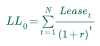 | |||||||||||||||||||||||||
Variants & steps (3)
What it meansDiscount lease payments at commencement. Use payments and the discount rate required by the applicable accounting standard.
Worked exampleSplit a lease payment between interest and liability reduction.
Worked exampleInitially recognize a right-of-use asset using the present value of lease payments, then separate financing-lease expense into interest and amortization. The simple initial measurement excludes prepayments, incentives and other initial adjustments; amortize the course example over its lease term.
Worked exampleSource Module | ||||||||||||||||||||||||||
Defined-benefit pension |  | |||||||||||||||||||||||||
Variants & steps (3)
What it meansMeasure the deficit or surplus of a defined-benefit pension plan. Positive means an unfunded net obligation; negative means a funded surplus. The reconciliation subtracts plan assets from the obligation, using a liability-positive sign. It assumes no asset-ceiling adjustment; a recognized pension asset may be limited under IFRS.
Worked exampleCalculate the IFRS net interest component of defined-benefit pension cost. A positive result is net interest expense; a negative result is net interest income. The simplified full-period calculation uses the beginning net balance and discount rate and assumes no contribution, benefit-payment or plan-change timing adjustments. Use the recognized balance after any applicable asset-ceiling limit.
Worked exampleCombine service cost and net interest to measure defined-benefit pension expense under IFRS; remeasurements are recognized in other comprehensive income. Remeasurements are reported in other comprehensive income, rather than this profit-or-loss expense.
Worked exampleSource Module | ||||||||||||||||||||||||||
Module 9 · Analysis of Income Taxes3 formulas | ||||||||||||||||||||||||||
Income tax expense and taxes paid |  | |||||||||||||||||||||||||
Variants & steps (2)
What it meansCombine current and deferred income tax expense. Exclude deferred-tax movements recorded outside the income statement.
Worked exampleReconcile income tax expense to cash taxes paid, adjusting current and deferred tax balances. Use deferred tax changes recognized in tax expense; exclude changes from acquisitions, other comprehensive income and other non-expense transactions.
Worked exampleSource Module | ||||||||||||||||||||||||||
Effective and cash tax rates | 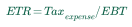 | |||||||||||||||||||||||||
Variants & steps (2)
What it meansRelate reported tax expense to accounting profit.
Worked exampleCompare cash taxes with pretax accounting income.
Worked exampleSource Module | ||||||||||||||||||||||||||
Deferred tax assets and liabilities | 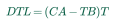 | |||||||||||||||||||||||||
Variants & steps (3)
What it meansMeasure tax on a positive taxable temporary asset difference.
Worked exampleMeasure a deductible temporary asset difference. Recognition depends on recoverability; use a positive deductible difference.
Worked exampleCompare a liability’s tax base with its carrying amount and apply the tax rate to identify the deferred tax liability or asset. Apply the liability-side temporary-difference rules, with the course’s recognition conditions for deferred tax assets.
Worked exampleSource Module | ||||||||||||||||||||||||||
Module 11 · Financial Analysis Techniques9 formulas | ||||||||||||||||||||||||||
Inventory, receivables and payables turnover and days | 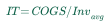 | |||||||||||||||||||||||||
Variants & steps (6)
What it meansMeasure how often inventory turns over.
Worked exampleExpress the inventory balance as the number of days of annual cost of goods sold it represents. A 365-day year, annual COGS, and average inventory. Use a different day count if a question specifies one.
Worked exampleMeasure collection efficiency using receivable balances.
Worked exampleTranslate receivable turnover into collection days.
Worked exampleMeasure supplier-payment turnover. Use purchases instead of COGS if the required convention specifies purchases.
Worked exampleTranslate payables turnover into payment days.
Worked exampleSource Module | ||||||||||||||||||||||||||
Working-capital, fixed-asset and total-asset turnover |  | |||||||||||||||||||||||||
Variants & steps (3)
What it meansMeasure sales generated per unit of working capital.
Worked exampleCompare sales with net fixed-asset investment.
Worked exampleMeasure the sales productivity of the asset base.
Worked exampleSource Module | ||||||||||||||||||||||||||
Liquidity ratios and defensive interval |  | |||||||||||||||||||||||||
Variants & steps (4)
What it meansCompare near-term assets with near-term obligations at a balance-sheet date. Use matching dates and units. A high ratio alone does not establish the quality or liquidity of the assets.
Worked exampleCompare readily available assets with current obligations.
Worked exampleAssess liquidity using cash and marketable investments alone.
Worked exampleEstimate the days of operations supported by liquid assets.
Worked exampleSource Module | ||||||||||||||||||||||||||
Interest and fixed-charge coverage |  | |||||||||||||||||||||||||
Variants & steps (2)
What it meansCompare earnings before interest and tax with interest expense.
Worked exampleAssess coverage of interest and included lease commitments. Use the specified lease accounting and expense basis.
Worked exampleSource Modules | ||||||||||||||||||||||||||
Return on assets (and variants) |  | |||||||||||||||||||||||||
Variants & steps (4)
What it meansRelate earnings to the average assets supporting them.
Worked exampleMeasure operating profitability of the asset base.
Worked exampleAdd back after-tax financing costs when comparing the return earned on assets. This after-tax alternative differs from net-income ROA and pretax operating ROA. Use the same definition consistently across companies and periods.
Worked exampleMeasure operating cash produced per unit of assets.
Worked exampleSource Module | ||||||||||||||||||||||||||
Return on equity (and variants) | 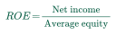 | |||||||||||||||||||||||||
Variants & steps (3)
What it meansRelate a period's earnings to the equity supporting those earnings. This example uses total net income and average total shareholders' equity consistently. Negative equity makes the conventional ratio difficult to interpret.
Worked exampleMeasure profit available to common owners relative to their equity.
Worked exampleCompare operating cash generation with owners' investment.
Worked exampleSource Module | ||||||||||||||||||||||||||
DuPont analysis (2-, 3-, 5-part) |  | |||||||||||||||||||||||||
Variants & steps (4)
What it meansSeparate profitability, asset efficiency, and financial leverage to explain ROE. Use consistent income, sales, average assets, and average equity across the three ratios.
Worked exampleSeparate return on assets from financial leverage.
Worked exampleSeparate tax, financing, margin, efficiency and leverage effects on ROE. NI/EBT is the tax burden; EBT/EBIT is the interest burden; EBIT/Sales is the EBIT margin; Sales/Assets is asset turnover; Assets/Equity is leverage.
Worked exampleMeasure the asset base supported by each unit of equity.
Worked exampleSource Module | ||||||||||||||||||||||||||
Industry-specific ratios |  | |||||||||||||||||||||||||
Variants & steps (11)
What it meansMeasure a bank's net interest earnings relative to earning assets.
Worked exampleCompare reserve holdings with the defined deposit base.
Worked exampleMeasure liquid securities relative to the required deposit base.
Worked exampleCompare retail sales productivity per unit of space.
Worked exampleMeasure revenue productivity of the workforce.
Worked exampleMeasure profit relative to workforce size.
Worked exampleMeasure room revenue per sold room night.
Worked exampleMeasure utilization of a hotel's room capacity.
Worked exampleMeasure revenue earned per user.
Worked exampleEvaluate underwriting costs relative to earned insurance premiums under the stated convention. This calculation uses earned premiums as the denominator; other reported combined ratios can use different expense-ratio bases. Below one indicates an underwriting profit on this basis, before investment income and other excluded items. Above one indicates an underwriting loss. Check the definition used by the insurer before comparing.
Worked exampleMeasure utilization of an airline's seat capacity.
Worked exampleSource Module | ||||||||||||||||||||||||||
Common-size statements | 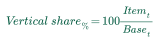 | |||||||||||||||||||||||||
Variants & steps (1)
What it meansCompare statement composition vertically or changes in an item over time. Vertical balance-sheet percentages use total assets. Vertical income-statement percentages normally use revenue; financial institutions sometimes use total assets, so label the chosen base. Horizontal analysis uses the same item in a base year or prior period. Use consistent accounting and currency bases; a zero comparison denominator is undefined. Percentage growth from a negative prior value can be misleading; the example requires a positive prior/base-year item.
Worked exampleSource Module | ||||||||||||||||||||||||||
Also used in this subject: QM · M1 · QM · M6 · FSA · M3 · FSA · M5 · EC · M1 · CF · M6 · FSA · M11 ·
| Formula | Equation | Details | ||||||||||||||||||
|---|---|---|---|---|---|---|---|---|---|---|---|---|---|---|---|---|---|---|---|---|
Module 2 · Equity Jurisdictions, Classes, and the Voting Process1 formula | ||||||||||||||||||||
Depositary receipt price | 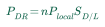 | |||||||||||||||||||
Variants & steps (1)
What it meansCompare receipt prices with the currency-adjusted underlying shares.
Worked exampleSource Module | ||||||||||||||||||||
Module 3 · Equity Issuance and Trading2 formulas | ||||||||||||||||||||
Bid-ask spread and mid-price | 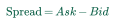 | |||||||||||||||||||
Variants & steps (3)
What it meansMeasure the quoted cost of crossing the market.
Worked exampleFind the midpoint of the best quoted prices.
Worked exampleExpress the quoted trading spread relative to the current lowest ask price. The denominator here is the ask price. The result is a fraction; multiply by 100 to express it as a percentage. Keep the price basis consistent when comparing spreads.
Worked exampleSource Module | ||||||||||||||||||||
VWAP, trading volume and turnover |  | |||||||||||||||||||
Variants & steps (3)
What it meansCompute an average price weighted by traded volume.
Worked exampleAverage trading activity over a stated period.
Worked exampleCompare market trading activity with investable shares.
Worked exampleSource Module | ||||||||||||||||||||
Module 4 · Sources of Equity Returns2 formulas | ||||||||||||||||||||
Dividend discount model (one-period and finite horizon) | 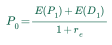 | |||||||||||||||||||
Variants & steps (2)
What it meansDiscount the expected dividend and resale proceeds.
Worked exampleValue dividends and a terminal sale on a consistent basis.
Worked exampleSource Module | ||||||||||||||||||||
Share repurchases and stock splits |  | |||||||||||||||||||
Variants & steps (2)
What it meansCalculate the number of shares removed through a repurchase. Use a constant or weighted-average repurchase price and consistent currency units. The simplified calculation excludes transaction fees.
Worked exampleAdjust per-share price and share count for a stock split. The reciprocal price and share-count changes leave total equity value unchanged in this mechanical adjustment. X must be positive; a reverse split has X below one. Actual market prices can move, and fractional-share cash settlements need separate treatment.
Worked exampleSource Module | ||||||||||||||||||||
Module 5 · Introduction to Equity Valuation2 formulas | ||||||||||||||||||||
Price-to-book (observed and justified) |  | |||||||||||||||||||
Variants & steps (4)
What it meansCompare market price with common book equity.
Worked exampleRelate a book multiple to profitability, growth and required return. Uses a stable-growth model and consistent beginning-book ROE; re exceeds g.
Worked exampleEstimate a peer-based book multiple from its drivers.
Worked exampleExpress common book equity per share.
Worked exampleSource Module | ||||||||||||||||||||
Residual income valuation | 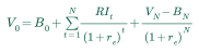 | |||||||||||||||||||
Variants & steps (2)
What it meansAdd discounted residual earnings to book equity. Uses clean-surplus accounting and consistent total or per-share quantities.
Worked exampleDeduct the required equity earnings charge.
Worked exampleSource Module | ||||||||||||||||||||
Module 6 · Discounted Cash Flow (DCF) and Growth Models5 formulas | ||||||||||||||||||||
Gordon growth model (value, implied return, implied growth) | 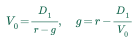 | |||||||||||||||||||
Variants & steps (4)
What it meansValue a stream of dividends growing at a constant rate indefinitely. D1 is next period's dividend, not the dividend just paid. The required return must exceed perpetual growth. Rearranging the same constant-growth relationship gives implied growth equal to required return minus the forward dividend yield, D1/value. Use the next expected dividend on the same horizon.
Worked exampleEstimate a forward market return using dividend yield and growth.
Worked exampleCalculate the compensation for expected market risk.
Worked exampleGrow the current dividend once before discounting a perpetual constant-growth dividend stream; required return must exceed growth.
Worked exampleSource Modules | ||||||||||||||||||||
FCFE valuation (multi-stage and terminal value) | 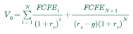 | |||||||||||||||||||
Variants & steps (5)
What it meansCombine explicit cash flows with a constant-growth terminal value. Required return must exceed terminal growth.
Worked exampleDiscount forecast equity cash flows and a terminal value estimated from a cash-flow multiple. The multiple here uses final forecast-year FCFE. In a constant-growth forecast, FCFEN=FCFE0(1+g)N. Match the valuation multiple to its cash-flow period; a forward multiple requires the corresponding forward cash flow.
Worked exampleSolve for growth implied by the residual terminal value.
Worked exampleValue equity cash flows at the forecast horizon. re must exceed g.
Worked exampleExpress stable-growth equity value as a cash-flow multiple.
Worked exampleSource Modules | ||||||||||||||||||||
FCFF valuation (firm value and terminal value) | 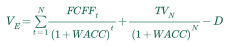 | |||||||||||||||||||
Variants & steps (3)
What it meansDiscount firm cash flow and subtract debt to obtain equity value. Add nonoperating assets and subtract other nonequity claims when relevant.
Worked exampleValue firm cash flow in a constant-growth model. WACC must exceed g.
Worked exampleExpress a constant-growth enterprise value as a cash-flow multiple.
Worked exampleSource Module | ||||||||||||||||||||
Sustainable growth, payout and retention |  | |||||||||||||||||||
Variants & steps (5)
What it meansLink dividend growth to retained earnings and equity profitability. Stable payout and return on reinvested equity; beginning-equity ROE differs from average-equity ROE.
Worked exampleLink operating reinvestment with return on capital.
Worked exampleMeasure earnings reinvested after net debt financing.
Worked exampleLink equity reinvestment and beginning-equity profitability to growth. Assumes stable returns on reinvested equity.
Worked exampleSeparate earnings distributed to owners from earnings retained. Use matching per-share bases and positive earnings for the conventional interpretation.
Worked exampleSource Module | ||||||||||||||||||||
Preferred stock value (perpetual and redeemable) | 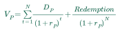 | |||||||||||||||||||
Variants & steps (2)
What it meansValue preferred shares with a specified redemption date.
Worked exampleValue a perpetual fixed preferred dividend.
Worked exampleSource Module | ||||||||||||||||||||
Module 7 · Relative Value Equity Valuation Approaches6 formulas | ||||||||||||||||||||
Enterprise value and market capitalization |  | |||||||||||||||||||
Variants & steps (2)
What it meansValue the operating business across funding claims.
Worked exampleCalculate the market value of the equity share class.
Worked exampleSource Module | ||||||||||||||||||||
PVGO and earnings yield | 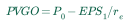 | |||||||||||||||||||
Variants & steps (2)
What it meansSeparate no-growth earnings value from growth-opportunity value.
Worked exampleConnect forward earnings yield with the growth portion of price.
Worked exampleSource Module | ||||||||||||||||||||
Price-to-sales (justified) | 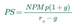 | |||||||||||||||||||
Variants & steps (1)
What it meansRelate a sales multiple to profit margin, payout and valuation rates.
Worked exampleSource Module | ||||||||||||||||||||
Price-to-earnings (observed, justified, PEG) |  | |||||||||||||||||||
Variants & steps (5)
What it meansExpress the share price as a multiple of earnings attributable to one share. State whether EPS is trailing or forward. This example uses positive trailing EPS.
Worked exampleValue next-period earnings under a stable-growth model. re must exceed g.
Worked exampleValue current earnings under a stable-growth dividend model. re must exceed g.
Worked exampleTranslate a revenue multiple into an earnings multiple using compatible profitability.
Worked exampleScale an earnings multiple by expected earnings growth. For 10% EPS growth, enter 10 in the growth field.
Worked exampleSource Module | ||||||||||||||||||||
Enterprise value multiples (EV/EBITDA, EV/capital) |  | |||||||||||||||||||
Variants & steps (7)
What it meansConnect an enterprise earnings multiple with cash conversion and valuation assumptions. EBITDA, taxes, capital spending and working-capital investment all refer to next period; WACC must exceed g.
Worked exampleCalculate an observed enterprise-value earnings multiple. This observed ratio differs from a model-implied justified multiple. State whether EBITDA is trailing, current-year or forward, and use consistent currency and accounting bases across peers. EBITDA must be positive for the conventional valuation-multiple interpretation; a zero denominator is undefined. Capitalization and lease policies can affect comparability.
Worked exampleCompare operating market value with operating book capital.
Worked exampleConnect enterprise value per unit of capital with profitability and reinvestment.
Worked exampleReconstruct operating earnings before noncash asset charges. Adjust for nonoperating items when the reporting definition requires it.
Worked exampleCompare operating enterprise value with the book value of invested capital, using consistent claims in numerator and denominator. This course value-to-book ratio does not subtract cash.
Worked exampleCompare enterprise value with revenue or a matching operating profit measure to value the whole business. State the chosen denominator; revenue, EBIT and EBITDA multiples have different interpretations.
Worked exampleSource Module | ||||||||||||||||||||
Dividend yield (trailing, forward, stable growth) |  | |||||||||||||||||||
Variants & steps (2)
What it meansInfer a dividend yield consistent with the Gordon model.
Worked exampleDistinguish the yield based on the recent dividend rate from the yield based on next-year dividend forecasts. Keep the dividend period and price date explicit. Both results are fractions; multiply by 100 for percentage yields.
Worked exampleSource Module | ||||||||||||||||||||
Module 8 · Financial Statement Forecasting in Equity Valuation3 formulas | ||||||||||||||||||||
Revenue, expense and finance-cost forecasting | 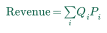 | |||||||||||||||||||
Variants & steps (8)
What it meansBuild revenue forecasts across product lines.
Worked exampleMeasure sales revenue at a given price and output.
Worked exampleProject expense changes using a historical linear relationship.
Worked exampleProject a cash flow growing at a constant rate.
Worked exampleProject sales with a stated growth assumption.
Worked exampleForecast interest income and expense from financial balances and interest rates. The source expense example applies the rate to beginning gross debt and describes forecasting interest income from cash and investments in the same way. Specify a beginning or representative balance consistent with the forecast timing; changing balances may require an average or time-weighted balance. Rates cover the modeled period. Other financing fees, tax effects and non-interest financial items are excluded.
Worked exampleForecast an asset item’s percentage change from revenue growth using an estimated intercept and sensitivity.
Worked exampleCombine volume growth and price growth, including their interaction, to estimate organic revenue growth.
Worked exampleSource Module | ||||||||||||||||||||
External financing need |  | |||||||||||||||||||
Variants & steps (1)
What it meansEstimate funding required after internal sources.
Worked exampleSource Module | ||||||||||||||||||||
Venture capital valuation (pre/post-money, ownership) |  | |||||||||||||||||||
Variants & steps (4)
What it meansReconcile company value before and after a financing round.
Worked exampleCalculate the ownership share implied by a financing round.
Worked exampleDiscount an equity exit value based on a sales multiple.
Worked exampleConvert a target annual IRR into a holding-period return multiple and discount the estimated exit value by that multiple.
Worked exampleSource Module | ||||||||||||||||||||
Module 12 · The Capital Asset Pricing Model, Market Model, and Other Factor-Based Equity Models6 formulas | ||||||||||||||||||||
Beta: estimation, portfolio beta, adjusted beta | 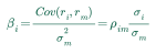 | |||||||||||||||||||
Variants & steps (4)
What it meansMeasure sensitivity to market risk.
Worked exampleMeasure market sensitivity rather than total volatility.
Worked exampleCombine systematic risk exposures using portfolio weights.
Worked exampleShrink a historical β estimate toward the market β of 1.
Worked exampleSource Modules | ||||||||||||||||||||
Unlevering and relevering beta | 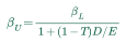 | |||||||||||||||||||
Variants & steps (2)
What it meansRemove leverage from a comparable firm's equity β. Assumes negligible debt β and the stated tax-shield model.
Worked exampleApply target financial leverage to an operating-risk β.
Worked exampleSource Module | ||||||||||||||||||||
Market (single-index) model and variance decomposition | 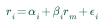 | |||||||||||||||||||
Variants & steps (5)
What it meansSeparate an asset return into market-related and residual components.
Worked exampleEstimate β and abnormal return from excess returns.
Worked exampleSeparate realized market exposure from asset-specific surprises.
Worked examplePredict fitted asset excess return from market excess return. This is the fitted characteristic line; observed returns can deviate from it.
Worked exampleDecompose risk when the market factor and residual are uncorrelated.
Worked exampleSource Modules | ||||||||||||||||||||
Country risk premium and cost of equity |  | |||||||||||||||||||
Variants & steps (2)
What it meansAdd a country-risk adjustment within the stated β-scaled model.
Worked exampleScale a sovereign spread to estimate an equity country-risk premium.
Worked exampleSource Module | ||||||||||||||||||||
Multifactor models | 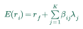 | |||||||||||||||||||
Variants & steps (3)
What it meansCombine multiple compensated risk exposures.
Worked exampleModel expected returns using several priced risk factors.
Worked exampleEstimate expected excess return using four factor premiums.
Worked exampleSource Module | ||||||||||||||||||||
CAPM / security market line | ![r_e = r_f + β [E(r_m) − r_f]](/resources/formula-equations/1ebc0e4dcd3321f6.svg) | |||||||||||||||||||
Variants & steps (1)
What it meansEstimate a required return using exposure to market risk. The equity risk premium is the expected market return minus the risk-free rate. It is not the market return itself.
2027 scope note: 2027 scope: Equities expands practical cost-of-equity estimation using market data. CAPM itself is not a new equation. Worked exampleSource Modules | ||||||||||||||||||||
| Formula | Equation | Details | ||||||||||||||||
|---|---|---|---|---|---|---|---|---|---|---|---|---|---|---|---|---|---|---|
Module 2 · Fixed-Income Cash Flows and Types1 formula | ||||||||||||||||||
Convertible bond conversion value and ratio |  | |||||||||||||||||
Variants & steps (2)
What it meansMeasure the equity value available through conversion.
Worked exampleCalculate shares delivered per convertible bond.
Worked exampleSource Module | ||||||||||||||||||
Module 4 · Fixed-Income Markets for Corporate Issuers1 formula | ||||||||||||||||||
Repo price, interest and margin |  | |||||||||||||||||
Variants & steps (4)
What it meansFind the maturity cash amount in a repo. For the ACT/360 convention used here, T is actual days divided by 360; use the agreement's day-count convention.
Worked exampleCompare repo collateral with cash funding. Notation: collateral value is the course security price; cash lent is the repo purchase price.
Worked exampleMeasure the collateral value excluded from funding.
Worked exampleCalculate the signed difference between required and posted repo collateral. A positive amount indicates a collateral shortfall; a negative amount indicates excess collateral that may be returned under the agreement.
Worked exampleSource Module | ||||||||||||||||||
Module 6 · Fixed-Income Bond Valuation: Prices and Yields2 formulas | ||||||||||||||||||
Bond price from yield (incl. coupon, YTC equation) | 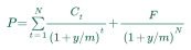 | |||||||||||||||||
Variants & steps (3)
What it meansDiscount each promised bond payment at the stated yield.
Worked exampleCalculate one periodic coupon payment.
Worked exampleSolve a callable bond's yield assuming exercise on the stated call date.
Worked exampleSource Modules | ||||||||||||||||||
Full price, accrued interest and flat price | 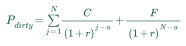 | |||||||||||||||||
Variants & steps (3)
What it meansValue a bond when settlement is between coupon dates.
Worked exampleConvert a quoted clean price into a settlement value.
Worked exampleAllocate a coupon to the accrued part of its period. Use the instrument's stated day-count convention.
Worked exampleSource Module | ||||||||||||||||||
Module 7 · Yield and Yield Spread Measures for Fixed-Rate Bonds2 formulas | ||||||||||||||||||
Current yield, simple yield and yield to worst | 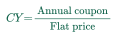 | |||||||||||||||||
Variants & steps (4)
What it meansCompare annual coupon income with the bond's clean price. Price and coupon refer to the same face amount. This omits reinvestment and any gain or loss at maturity.
Worked exampleEstimate a simple income-plus-amortization yield. This convention is an approximation and differs from compound YTM.
Worked exampleIdentify the lowest relevant yield under the quoted call convention.
Worked exampleConvert a 30/360 annual yield to an ACT/ACT basis using the course’s 365/360 adjustment. The course conversion uses 365 days for the actual annual basis.
Worked exampleSource Module | ||||||||||||||||||
Yield spreads (G, I, Z, OAS) and option-adjusted price |  | |||||||||||||||||
Variants & steps (5)
What it meansMeasure a bond's yield premium to a government benchmark.
Worked exampleCompare a bond yield with its swap-curve benchmark.
Worked exampleFind the constant spread that reprices cash flows on a spot curve. Rates use the same per-period compounding convention.
Worked exampleAdd back the issuer call option to obtain an option-adjusted bond price. Use otherwise comparable bonds and the same price basis. The issuer owns the call, so its value reduces the investor value of the callable bond. The embedded-option value depends on the option model and interest-rate volatility assumptions; the calculator takes that model value as an input.
Worked exampleRemove the embedded option cost from the Z-spread to compare bonds after adjusting for optionality. Both quantities must be expressed as annualized spread basis points; the option cost is not a cash option premium.
Worked exampleSource Module | ||||||||||||||||||
Module 8 · Yield and Yield Spread Measures for Floating-Rate Instruments2 formulas | ||||||||||||||||||
Floating-rate note coupon and price |  | |||||||||||||||||
Variants & steps (2)
What it meansDetermine the next coupon rate of a floating-rate instrument. Notation: QM is the quoted margin, the issuer-specific credit spread added to the reference rate.
Worked exampleValue a floater under a constant reference-rate scenario.
Worked exampleSource Module | ||||||||||||||||||
Money market yields (discount and add-on) |  | |||||||||||||||||
Variants & steps (4)
What it meansAnnualize a discount as a fraction of face value.
Worked examplePrice an instrument whose quote uses a face-value discount convention.
Worked exampleAnnualize a discount relative to the amount invested.
Worked examplePrice a money-market instrument from its investment-based yield.
Worked exampleSource Module | ||||||||||||||||||
Module 9 · The Term Structure of Interest Rates: Spot, Par, and Forward Curves2 formulas | ||||||||||||||||||
Spot rates, discount factors and par rate |  | |||||||||||||||||
Variants & steps (3)
What it meansDiscount cash flows on their own maturity-specific spot rates.
Worked exampleConvert a spot yield into a present-value multiplier.
Worked exampleFind the coupon per unit face value that makes a bond trade at par. Multiply by payment frequency for a nominal annual quote.
Worked exampleSource Module | ||||||||||||||||||
Implied forward rates | ![f_(A, B) = [((1 + z_B )^B) / ((1 + z_A )^A)]^(1/(B − A)) − 1](/resources/formula-equations/05d7e3cf2920c11b.svg) | |||||||||||||||||
Variants & steps (1)
What it meansFind the annual forward rate between two maturities. B must exceed A. Notation: the forward rate corresponds to the course’s implied forward rate IFR for the same start date and horizon.
Worked exampleSource Modules | ||||||||||||||||||
Module 10 · Interest Rate Risk and Return2 formulas | ||||||||||||||||||
Macaulay duration (incl. special cases, duration gap) | 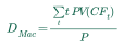 | |||||||||||||||||
Variants & steps (7)
What it meansFind the present-value-weighted time to cash receipts.
Worked exampleCalculate duration in coupon periods for a fixed-coupon bond. Divide by payments per year for years; r=0 requires the limiting form.
Worked exampleCalculate fixed-coupon bond duration in years without a full cash-flow table. Nonzero periodic yield; equally spaced coupons and redemption at par.
Worked exampleMeasure duration for a level perpetuity. Divide by payment frequency to express years.
Worked exampleMeasure duration of a single fixed maturity payment.
Worked exampleApproximate a par floater's duration to its next rate reset. The result is in years: divide the remaining reset-period fraction by the number of resets per year. Assumes stable margin and minimal credit effects.
Worked exampleCompare Macaulay duration with the investment horizon to assess the balance between reinvestment risk and price risk.
Worked exampleSource Module | ||||||||||||||||||
Bond carrying value (amortized cost) |  | |||||||||||||||||
Variants & steps (1)
What it meansReconcile carrying value along the constant-yield bond price trajectory. Discount amortization raises carrying value toward par; premium amortization lowers it toward par. Use cumulative amortization from acquisition and a consistent quote basis. This simple relation excludes impairment, currency movements and other adjustments; add accrued interest separately when required by the price basis.
Worked exampleSource Module | ||||||||||||||||||
Module 11 · Yield-Based Bond Duration Measures and Properties2 formulas | ||||||||||||||||||
Modified duration and percentage price change |  | |||||||||||||||||
Variants & steps (4)
What it meansTranslate cash-flow timing into first-order sensitivity to a change in yield. Macaulay duration is in years; r is nominal annual yield compounded m times. Use the same yield convention throughout.
Worked exampleEstimate annualized price sensitivity by repricing fixed cash flows. Dmod here is annualized modified duration (AnnModDur in the course); Δy is an annualized yield shift.
Worked exampleApproximate a bond's percentage price move for a small yield change. Ignores convexity and assumes unchanged cash flows. One basis point is 0.01 percentage point.
Worked exampleConvert annual modified duration to annual Macaulay duration using the periodic yield and compounding frequency. Use the coupon-period yield r; annual durations are both measured in years.
Worked exampleSource Module | ||||||||||||||||||
Money duration and PVBP |  | |||||||||||||||||
Variants & steps (3)
What it meansExpress yield sensitivity in currency units.
Worked exampleEstimate the price change associated with one basis point.
Worked exampleEstimate the monetary price change for a small yield change; a yield increase produces a price decrease.
Worked exampleSource Module | ||||||||||||||||||
Module 12 · Yield-Based Bond Convexity and Portfolio Properties2 formulas | ||||||||||||||||||
Convexity and duration-convexity price change | 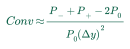 | |||||||||||||||||
Variants & steps (4)
What it meansEstimate annualized second-order yield sensitivity.
Worked exampleExpress second-order yield sensitivity in currency units.
Worked exampleImprove a duration-only approximation for larger yield changes.
Worked exampleAdd the money-convexity correction to the money-duration estimate for a larger yield change.
Worked exampleSource Module | ||||||||||||||||||
Portfolio duration and convexity |  | |||||||||||||||||
Variants & steps (2)
What it meansApproximate portfolio sensitivity under a parallel yield shift.
Worked exampleCombine second-order sensitivities across a bond portfolio.
Worked exampleSource Module | ||||||||||||||||||
Module 13 · Curve-Based and Empirical Fixed-Income Risk Measures2 formulas | ||||||||||||||||||
Effective duration and convexity | 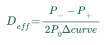 | |||||||||||||||||
Variants & steps (3)
What it meansMeasure sensitivity when expected cash flows can change with rates.
Worked exampleMeasure second-order curve sensitivity including changing cash flows.
Worked exampleEstimate percentage price change from a parallel benchmark-curve shift, allowing expected cash flows to change.
Worked exampleSource Module | ||||||||||||||||||
Key rate duration | 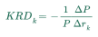 | |||||||||||||||||
Variants & steps (3)
What it meansMeasure exposure to a specific yield-curve maturity.
Worked exampleEstimate price impact from a nonparallel curve change.
Worked exampleSum sensitivities to individual benchmark maturities to recover effective duration for a parallel curve shift. For the course’s complete set of key rates and a consistent parallel curve shift.
Worked exampleSource Module | ||||||||||||||||||
Module 14 · Credit Risk1 formula | ||||||||||||||||||
Expected loss, LGD and credit spread |  | |||||||||||||||||
Variants & steps (4)
What it meansEstimate average credit loss over a consistent horizon.
Worked exampleConvert recovery assumptions into conditional currency loss.
Worked exampleEstimate compensation for expected default loss. The credit spread approximation uses loss given default normalized per unit of exposure: LGD = 1 − recovery rate. Multiplying by default probability gives a spread fraction, rather than a currency loss.
Worked exampleEstimate the percentage price impact of a credit-spread change while holding the benchmark curve constant.
Worked exampleSource Module | ||||||||||||||||||
Module 15 · Credit Analysis for Government Issuers2 formulas | ||||||||||||||||||
Sovereign debt and interest burden ratios |  | |||||||||||||||||
Variants & steps (4)
What it meansAssess a sovereign's debt burden relative to its economy.
Worked exampleCompare sovereign obligations with recurring public revenue.
Worked exampleMeasure interest-service burden relative to economic output.
Worked exampleMeasure the share of public revenue absorbed by interest.
Worked exampleSource Module | ||||||||||||||||||
Sovereign economic and external ratios |  | |||||||||||||||||
Variants & steps (7)
What it meansCompare economic output per person.
Worked exampleMeasure inflation-adjusted economic growth.
Worked exampleCompare external liquidity with the size of an economy.
Worked exampleCompare reserve assets with foreign-creditor obligations.
Worked exampleMeasure structural external indebtedness.
Worked exampleAssess near-term external refinancing pressure.
Worked exampleMeasure the sample dispersion of real GDP growth as an indicator of business-cycle variability. The course identifies standard deviation as the volatility metric. This example explicitly uses the sample convention.
Worked exampleSource Module | ||||||||||||||||||
Module 16 · Credit Analysis for Corporate Issuers1 formula | ||||||||||||||||||
Corporate credit ratios |  | |||||||||||||||||
Variants & steps (2)
What it meansCompare borrowing with an operating cash-earnings proxy.
Worked exampleCompare retained cash generation with debt net of liquid assets.
Worked exampleSource Modules | ||||||||||||||||||
Module 18 · Asset-Backed Security (ABS) Instrument and Market Features1 formula | ||||||||||||||||||
Overcollateralization (and excess spread) | 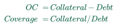 | |||||||||||||||||
Variants & steps (2)
What it meansMeasure excess assets supporting an ABS structure. Distinguish collateral-to-debt coverage from an excess-collateral percentage.
Worked exampleSubtract the security coupon from the collateral coupon to measure the interest margin available as credit support.
Worked exampleSource Module | ||||||||||||||||||
Module 19 · Mortgage-Backed Security (MBS) Instrument and Market Features3 formulas | ||||||||||||||||||
Mortgage pool WAC, WAM and pass-through rate |  | |||||||||||||||||
Variants & steps (3)
What it meansWeight mortgage coupon rates by current principal balances.
Worked exampleFind the principal-weighted remaining maturity of a mortgage pool.
Worked exampleCalculate the net coupon passed from a mortgage pool to security holders. Express the pool coupon and all deducted fees on the same annual rate basis. This simple pass-through convention does not describe the coupon rules of every structured mortgage tranche, nor does it fix principal or prepayment timing.
Worked exampleSource Module | ||||||||||||||||||
Loan-to-value and debt-to-income |  | |||||||||||||||||
Variants & steps (2)
What it meansMeasure the mortgage balance relative to collateral value.
Worked exampleAssess a borrower's monthly debt-service capacity.
Worked exampleSource Module | ||||||||||||||||||
NOI and debt service coverage |  | |||||||||||||||||
Variants & steps (2)
What it meansBuild the property income used in debt-service coverage. Use the specific transaction's definition; exclude mortgage interest and principal.
Worked exampleMeasure a property's capacity to meet its borrowing commitments.
Worked exampleSource Module | ||||||||||||||||||
| Formula | Equation | Details | ||||||||||||||||||
|---|---|---|---|---|---|---|---|---|---|---|---|---|---|---|---|---|---|---|---|---|
Module 2 · Forward Commitment and Contingent Claim Features and Instruments1 formula | ||||||||||||||||||||
Option payoff and profit |  | |||||||||||||||||||
Variants & steps (8)
What it meansMeasure the exercise value of a purchased call.
Worked exampleInclude the initial call premium in expiry profit. Ignores the financing cost of the premium.
Worked exampleMeasure the exercise value of a purchased put.
Worked exampleInclude the premium in a long put's expiry profit. Ignores the financing cost of the premium.
Worked exampleEvaluate the obligation of a put writer.
Worked exampleEvaluate the obligation of a call writer.
Worked exampleAdd the premium paid to the exercise price to find the underlying price at which a long call’s expiry profit is zero.
Worked exampleCompare a call with a forward by setting the call’s exercise price equal to the original forward price; subtract the call premium from its payoff.
Worked exampleSource Modules | ||||||||||||||||||||
Module 4 · Arbitrage, Replication, and the Cost of Carry in Pricing Derivatives1 formula | ||||||||||||||||||||
Forward price (cost of carry) |  | |||||||||||||||||||
Variants & steps (5)
What it meansPrice a forward on a non-income-producing asset.
Worked examplePrice a forward under continuous compounding.
Worked exampleAdjust a forward price for known income and carrying costs.
Worked examplePrice continuously accruing costs and benefits. All yields use a consistent continuous basis.
Worked exampleCombine financing, storage and holding benefits in a continuous-carry model.
Worked exampleSource Module | ||||||||||||||||||||
Module 5 · Pricing and Valuation of Forward Contracts and for an Underlying with Varying Maturities2 formulas | ||||||||||||||||||||
Forward contract value (incl. currency forward) | 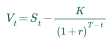 | |||||||||||||||||||
Variants & steps (6)
What it meansMark a forward to market when the underlying has no carry cash flows. Notation: K is the delivery price agreed at inception, written F0(T) in the course.
Worked exampleValue the short side of a forward without income or costs. Notation: K is the delivery price agreed at inception, written F0(T) in the course.
Worked exampleInclude only cash flows remaining until delivery. Notation: K is the delivery price agreed at inception, written F0(T) in the course.
Worked exampleIdentify the initial value when the delivery price equals the no-arbitrage forward price.
Calculate settlement on a long forward position.
Worked exampleValue a long forward in price currency f for each unit of base currency d using the course’s carry-adjusted convention. Course Module 5, Equation 9, gives value per unit of base currency using this carry-adjusted convention. Multiplying this course value by the base-currency discount factor gives the strictly discounted cash-flow value.
Worked exampleSource Module | ||||||||||||||||||||
FRA settlement and implied forward rate |  | |||||||||||||||||||
Variants & steps (2)
What it meansValue the interest difference when an FRA settles at the start of its accrual period. This is the undiscounted net payment over the accrual period. For cash settlement at the start, discount this payment at the reset market reference rate; the course gives both conventions.
Worked exampleFind the break-even forward reinvestment rate that links short- and long-maturity zero rates. First convert quoted APRs to a common compounding frequency; this example then uses annual effective rates.
Worked exampleSource Module | ||||||||||||||||||||
Module 6 · Pricing and Valuation of Futures Contracts2 formulas | ||||||||||||||||||||
Futures margin and daily settlement |  | |||||||||||||||||||
Variants & steps (2)
What it meansCalculate a long futures position's daily variation margin. A short position has the opposite sign; use the contract's quotation multiplier.
Worked exampleTrack variation margin before deposits or withdrawals.
Worked exampleSource Module | ||||||||||||||||||||
Interest rate futures quote and BPV |  | |||||||||||||||||||
Variants & steps (2)
What it meansConvert a short-term market reference rate into its 100-minus-rate futures quote. Enter the quoted reference rate as a percentage: 5 means 5%. This linear quote is an index convention, not the present value of a zero-coupon bond. Negative reference rates produce quotes above 100.
Worked exampleConvert a one-basis-point rate change into the contract value change. Applies to the fixed linear price-yield convention of short-term rate futures. Use the underlying deposit accrual period, not time until the futures expiry. A three-month period on a 90/360 basis has τ=0.25.
Worked exampleSource Module | ||||||||||||||||||||
Module 7 · Pricing and Valuation of Interest Rate and Other Swaps1 formula | ||||||||||||||||||||
Interest rate swap rate and value |  | |||||||||||||||||||
Variants & steps (4)
What it meansSet fixed and floating leg values equal at inception. The course uses equally spaced annual payments; the fixed rate is per annual payment period.
Worked exampleCalculate the net interest payment at a payment date.
Worked exampleMark a receive-floating, pay-fixed swap to market.
Worked exampleWeight the course’s equal-period forward rates by their discount factors to find the fixed swap rate with zero initial value. The course assumes equal annual payment periods, so the weights are discount factors.
Worked exampleSource Module | ||||||||||||||||||||
Module 8 · Pricing and Valuation of Options1 formula | ||||||||||||||||||||
Option exercise value, time value and bounds |  | |||||||||||||||||||
Variants & steps (4)
What it meansSeparate a European option premium into course-defined exercise value and time value. Course Module 8 uses the present value of the exercise price. The expiry payoff in Module 2 uses the exercise price without discounting; the two conventions refer to different times.
Worked exampleCheck call prices for basic no-arbitrage bounds. For a European call on a non-income-paying underlying with positive remaining maturity. Course Module 8 uses a strict lower inequality away from boundary cases; the limiting lower value is shown here.
Worked exampleCheck European put prices for basic no-arbitrage bounds. For a European put on a non-income-paying underlying, positive interest and positive remaining maturity, PV(X) is the tighter no-arbitrage upper bound. Course Module 8 instead states X as an upper bound; the two bounds coincide at expiry. The displayed lower limit is approached at the boundary. An American put has an upper bound equal to the undiscounted exercise price X.
Worked exampleApply the course’s present-value exercise-price convention to measure a European option’s exercise value before expiry. Course Module 8 discounts the exercise price; this is different from an expiry payoff.
Worked exampleSource Module | ||||||||||||||||||||
Module 9 · Option Replication Using Put–Call Parity1 formula | ||||||||||||||||||||
Put-call parity and synthetic positions | 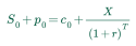 | |||||||||||||||||||
Variants & steps (7)
What it meansCompare a protective put with a fiduciary call. Same underlying, strike and expiry; no underlying income.
Worked exampleReplicate a European put from a call, cash and a short underlying.
Worked exampleReplicate the underlying using same-strike European options and cash.
Worked exampleRelate a covered call to cash less a put obligation.
Worked exampleApply parity to a forward exposure instead of spot ownership.
Worked exampleInterpret risky debt and equity as option-based claims.
Worked exampleCompare a put and call with the same strike and maturity using the discounted difference between strike and forward price.
Worked exampleSource Module | ||||||||||||||||||||
Module 10 · Valuing a Derivative Using a One-Period Binomial Model1 formula | ||||||||||||||||||||
One-period binomial option model | 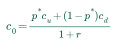 | |||||||||||||||||||
Variants & steps (5)
What it meansDiscount the risk-neutral expected option payoff.
Worked exampleExpress next-period prices as gross growth factors.
Worked exampleFind shares required to replicate one option.
Worked exampleValue an option from the stock position and its risk-free financing.
Worked exampleChoose probabilities that reproduce the risk-free expected underlying return. Requires d < 1 + r < u; p* is a pricing probability, not a forecast. Notation: u and d are gross price factors, corresponding to course Ru and Rd; subtract one to obtain net returns.
Worked exampleSource Module | ||||||||||||||||||||
| Formula | Equation | Details | ||||||||||||
|---|---|---|---|---|---|---|---|---|---|---|---|---|---|---|
Module 1 · Alternative Investment Features, Methods, and Structures1 formula | ||||||||||||||
Distribution waterfall: hurdle and catch-up | 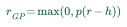 | |||||||||||||
Variants & steps (3)
What it meansCalculate an incentive on return above the hurdle. Notation: beginning and ending values correspond to course P0 and P1; management and hurdle rates to rm and rh; the high-water mark to PHWM.
Worked exampleApply a full GP catch-up after investors receive the hurdle. For a 100% catch-up tier, c = p·h/(1−p). The default 2% catch-up satisfies that relationship for p = 20% and h = 8%. Course Equation 2 applies to the segment where the return r exceeds hurdle h plus catch-up c (r > h + c). Notation: beginning and ending values correspond to course P0 and P1; management and hurdle rates to rm and rh; the high-water mark to PHWM.
Worked exampleOnce the soft hurdle is exceeded, apply the incentive fee to the whole eligible gain rather than only the gain above the hurdle. Once the soft hurdle is exceeded, the incentive share applies to the full return; below the hurdle there is no incentive allocation. Notation: beginning and ending values correspond to course P0 and P1; management and hurdle rates to rm and rh; the high-water mark to PHWM.
Worked exampleSource Module | ||||||||||||||
Module 2 · Alternative Investment Performance and Returns2 formulas | ||||||||||||||
Management and incentive fees, HWM and net return |  | |||||||||||||
Variants & steps (5)
What it meansCompute fees when the incentive is calculated before deducting management fees. Notation: beginning and ending values correspond to course P0 and P1; management and hurdle rates to rm and rh; the high-water mark to PHWM.
Worked exampleCompute an incentive after first deducting management fees. Notation: beginning and ending values correspond to course P0 and P1; management and hurdle rates to rm and rh; the high-water mark to PHWM.
Worked exampleApply a hard hurdle after the management fee deduction. Notation: beginning and ending values correspond to course P0 and P1; management and hurdle rates to rm and rh; the high-water mark to PHWM.
Worked exampleCharge an incentive only on net value above the contract's high-water mark. Notation: beginning and ending values correspond to course P0 and P1; management and hurdle rates to rm and rh; the high-water mark to PHWM.
Worked exampleMeasure the investor's net return with no external cash flows. Notation: beginning and ending values correspond to course P0 and P1; management and hurdle rates to rm and rh; the high-water mark to PHWM.
Worked exampleSource Module | ||||||||||||||
Multiple of invested capital |  | |||||||||||||
Variants & steps (1)
What it meansCompare total investment value with capital put to work. This multiple does not reflect cash-flow timing.
Worked exampleSource Module | ||||||||||||||
| Formula | Equation | Details | ||||||||||||
|---|---|---|---|---|---|---|---|---|---|---|---|---|---|---|
Module 1 · Portfolio Risk and Return: Part I3 formulas | ||||||||||||||
Equal-weight diversification and diversification ratio | 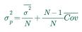 | |||||||||||||
Variants & steps (5)
What it meansIllustrate diversification as the asset count grows.
Worked exampleCompare diversification for assets with identical variances and correlations.
Worked exampleSeparate diversifiable and shared risk under equal variances.
Worked exampleCompare equal-weight portfolio risk with a comparable single-security benchmark. Compare portfolio volatility with the average single-stock volatility from a random-security selection. Lower values indicate more risk reduction on this convention. This portfolio-to-single-security ratio is the reciprocal of some other published diversification-ratio conventions; keep the definition and observation horizon explicit.
Worked exampleEstimate the limiting variance of a large equal-weight portfolio: idiosyncratic variance diversifies away, while average covariance remains. Equal asset volatilities, equal weights and a stable average pairwise correlation.
Worked exampleSource Module | ||||||||||||||
Adding a candidate asset (Sharpe condition) | ![E(R_new )_boundary = R_f + (σ_new ρ_(new, p)) / (σ_p)[E(R_p) − R_f], SR_new > SR_p ρ_(new, p)](/resources/formula-equations/8780e8ef90d0cd29.svg) | |||||||||||||
Variants & steps (1)
What it meansCompare expected return with the asset's contribution to portfolio risk. The equality gives the return boundary. With positive volatilities, a candidate return above it is equivalent to SRnew>SRp×correlation. This is a marginal mean-variance improvement condition for a small positive allocation, before transaction costs; it does not specify an optimal allocation.
Worked exampleSource Module | ||||||||||||||
Sharpe ratio and M-squared | 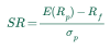 | |||||||||||||
Variants & steps (2)
What it meansCompare excess return per unit of total risk. Use realized average returns and measured volatility for an ex-post ratio.
Worked exampleExpress risk-adjusted performance at the market's volatility.
Worked exampleSource Modules | ||||||||||||||
Module 2 · Portfolio Risk and Return: Part II2 formulas | ||||||||||||||
Capital allocation line / capital market line | 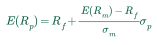 | |||||||||||||
Variants & steps (4)
What it meansDescribe efficient portfolios on the market allocation line. Assumes common borrowing and lending rates and nonnegative market exposure.
Worked exampleCompute total risk when the remaining weight earns a constant risk-free return.
Worked exampleRelate expected return to risk along a risk-free and risky-portfolio combination. Assumes the same lending and borrowing rate.
Worked examplePrice the return-risk trade-off after borrowing to buy the market.
Worked exampleSource Module | ||||||||||||||
Treynor ratio, Jensen's alpha and appraisal ratio | 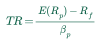 | |||||||||||||
Variants & steps (4)
What it meansCompare excess return per unit of market risk. Interpret cautiously for zero or negative β.
Worked exampleMeasure realized return above the CAPM benchmark. Portfolio, market and risk-free returns must use the same horizon.
Worked exampleMeasure abnormal return per unit of nonsystematic risk added to a diversified portfolio. This α-to-residual-volatility measure uses model α and residual volatility measured over the same period.
Worked exampleCompare the return-to-risk inputs described in the CAPM portfolio-construction discussion. The course allocation formula uses the expected market return. Treynor–Black versions may use market excess return; keep the chosen convention consistent.
Worked exampleSource Module | ||||||||||||||
Module 3 · Portfolio Management: An Overview1 formula | ||||||||||||||
Fund NAV per share |  | |||||||||||||
Variants & steps (1)
What it meansValue each fund share from net fund assets. Use consistent currency units and a common valuation time. A closed-end fund can trade above or below this NAV; NAV is an accounting value rather than a guarantee of its market price.
Worked exampleSource Module | ||||||||||||||
Practise identifying the relevant standard, the facts that matter, and the appropriate action.
Explore 186 formulas from Quizara's 2027 Level I course, with variants, conditions and source Modules. Use this study aid alongside your lessons; Ethics covers concepts and professional judgment.
Free for 14 days. No card required.
Explore 186 formulas with variants, conditions and source Modules. Change inputs in the calculators; 27 worked examples also include BA II Plus steps.
Every formula in this catalog is visible on this page without an account. Create a free Quizara account to unlock the PDF download, then return to this tab for it to start automatically. The PDF contains all the formulas currently listed here, with a contents page, variables, usage notes and the original worked examples.
Ethical and Professional Standards is a judgment subject. Practise identifying the relevant standard, the facts that matter and the appropriate action.
It marks a coverage change in Quizara's 2027 course. The equation itself may be unchanged.
Register in a new tab, then return here — your PDF will start downloading automatically.
![r_G = [∏_(t = 1)^(N) (1 + r_t)]^(1/N) − 1](/resources/formula-equations/6638ff1d679b5fe6.svg)




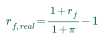

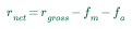

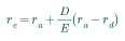


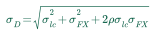
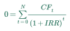


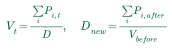




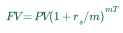



![APR_n = n[(1 + APR_m /m)^(m/n) − 1]](/resources/formula-equations/4605024378caf30f.svg)
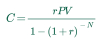
](/resources/formula-equations/5d90c2f809b1266c.svg)
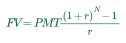
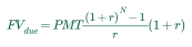
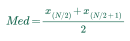
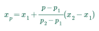

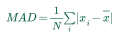

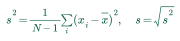
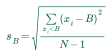
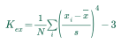

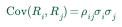
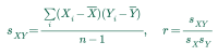

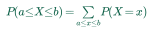

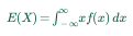





![E[r_P] = ∑_(i) p_i r_(P, i), σ_P^2 = ∑_(i) p_i(r_(P, i) − E[r_P])^2](/resources/formula-equations/e890b25344736392.svg)
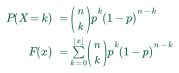



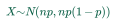
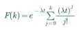


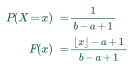
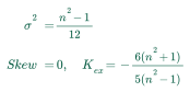


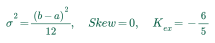
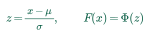

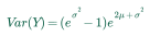
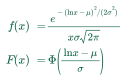
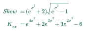
![E[ ln S_T] = ln S_0 + (μ − σ^2 /2) T, σ_T = σsqrt(T)](/resources/formula-equations/38645eacc169f15f.svg)
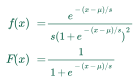





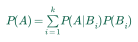

![Var(X∣Y) = E(X^2∣Y) − [E(X∣Y) ]^2](/resources/formula-equations/399b08e3a16e016c.svg)

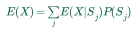
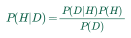


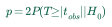



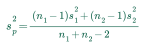

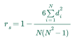


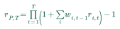
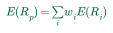
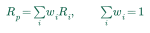

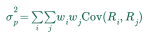





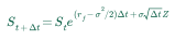


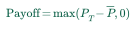


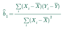

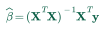
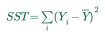
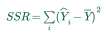
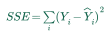


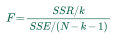

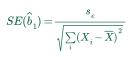
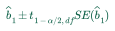
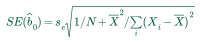


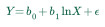
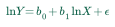




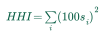


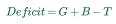

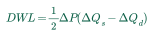

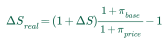


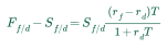
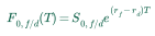
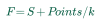
![(E_t[S_(f/d, t + 1)]) / (S_(f/d, t)) − 1 = (r_f − r_d) / (1 + r_d)](/resources/formula-equations/4709553980d6ef42.svg)
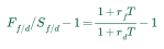

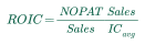
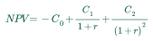








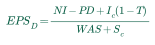
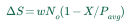







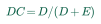

















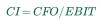
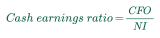








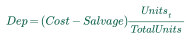









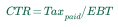
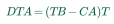

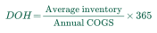
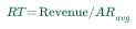

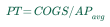


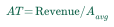
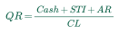



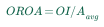
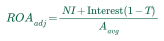




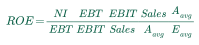



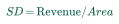





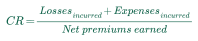
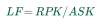
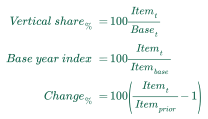

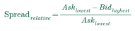


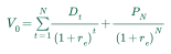
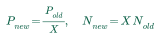



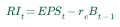

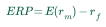

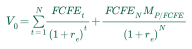
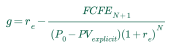

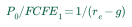


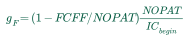
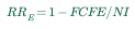
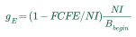




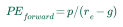
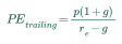
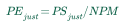

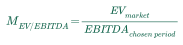
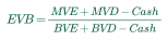
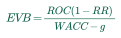



![Yield_trailing = (D_(annualized, recent)) / (P_t), Yield_forward = (E_t[D_(next year)]) / (P_t)](/resources/formula-equations/4b99d273834ed701.svg)


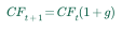

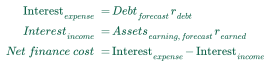



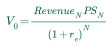

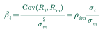

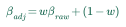
![β_L = β_U[1 + (1 − T) D/E]](/resources/formula-equations/ab95a61d80b77d0e.svg)


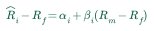

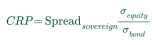
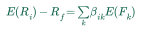






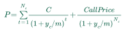
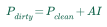

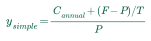

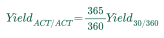

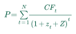


![P = ∑_(t = 1)^(N) (F(MRR + QM) /m) / ([1 + (MRR + DM) /m]^t) + (F) / ([1 + (MRR + DM) /m]^N)](/resources/formula-equations/a8ecf156a3dd1d34.svg)
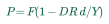




![D_period = (1 + r) / (r) − (1 + r + N(c − r)) / (c[(1 + r)^N − 1] + r) − a](/resources/formula-equations/49a4d7802165db0e.svg)
![D_Mac = (1) / (m)[(1 + r) / (r) − (1 + r + N(c − r)) / (c[(1 + r)^N − 1] + r) − a]](/resources/formula-equations/4aa7a849808be98d.svg)


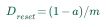

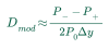
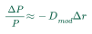

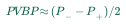


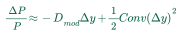

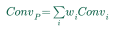
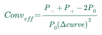

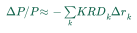
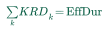






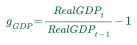




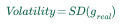




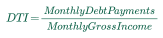




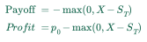
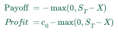



^T](/resources/formula-equations/1a7fabfcd1c4dea8.svg)


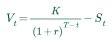
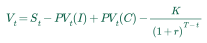


![V_t = S_(f/d, t) − F_(0, f/d) exp [ − (r_f − r_d)(T − t)]](/resources/formula-equations/c0aef1447be34ff8.svg)






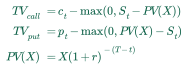



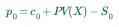
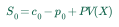
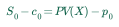

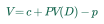
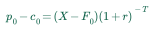


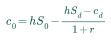

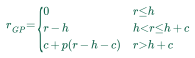





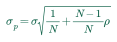
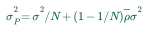
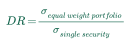

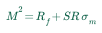

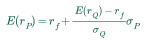
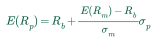
![α_p = R_p − [R_f + β_p(R_m − R_f)]](/resources/formula-equations/919a3415869beefa.svg)